Querying and Data Transformations
Table of contents
- Querying With Flux
- Flux Data Transformations
- Grouping
- Windowing
- Windowing and aggregateWindow()
- Real World Data Example of Grouping
- Aggregations
- Yielding
- Pivoting
- Mapping
- Returning values and arrays
- Reducing
- Manipulating Time
- Regex
- The String Package
- Combining Data Streams
- Accessing External Data Sources
- Materialized Views or Downsampling Tasks
- Further Reading
Querying With Flux
In the vernacular of Flux, a Flux script is called a “query.” This is despite the fact that you can write valid and useful Flux that doesn’t even query your own data at all. For our purposes now, we can think of writing a query as retrieving targeted data from the storage engine, as opposed to transforming and shaping the data, which will be discussed in detail in the following sections.
As described in the section “Just Enough Flux” in the previous chapter, you can see that a typical simple query involves 3 parts:
- The source bucket
- The range of time
- A set of filters
Additionally, a query may contain a yield() statement depending on circumstances.
from()
In most cases, a query starts by specifying a bucket to query from using the bucket name:
from(bucket: "bucket1")
In some cases, you may wish to use the bucket’s id instead:
from(bucketID: "497b48e409406cc7")
Typically, developers will address a bucket by its name for a few reasons. First, of course the bucket name is much more readable, the role of the bucket can be encoded in the name. Additionally, there may be times when deleting a bucket and creating a new one with the same name is the most expedient way to delete data. Addressing the bucket by its id has the advantage of being immutable. Someone can change the bucket name, and the query using the id will continue working.
There are cases that will be described below where you use a different kind of “from”, for example sql.from() or csv.from() or array.from() to bring in data from other sources.
range()
The range function is required directly after from()and its purpose is to specify the points to include based on their timestamps. range() has only two parameters.
start and stop
An argument for start is required, whereas stop is optional. In the case where you leave out an argument for stop, Flux will substitute now(), which is the current time when execution is scheduled.
now()
now() always returns the time when a Flux script is scheduled to start execution. This has some important implications:
- If your script is not run as part of a task, now() will return the time at the very start of execution of the script. If there are any delays, for example due to queuing as a result of excessive load, etc… now() will the time when the script was scheduled to run.
- If your script is running as part of a task, now() will return the time that your script was scheduled to run.
- Every call to now() in the script will return the same time.
Calling range() with Relative Durations
Possibly the most common way to use the range function is to use a start time like this:
range(start: -5m)
This says to provide all of the data that is available starting five minutes ago. This is inclusive, meaning that any data that is timestamped exactly with the nanosecond exactly five minutes ago will be included. Any data that is five minutes and one nanosecond older or more will not be included.
Conversely, stop is exclusive. That is to say that if you have any data that is timestamped exactly with the stop argument, it will NOT be included with the results.
So, for example, if there is data that is timestamped precisely 1 minute ago, and you have the following queries, that data will be included in the second query, but not the first.
from(bucket: "bucket1")
|> range(start: -2m, stop: -1m)

from(bucket: "bucket1")
|> range(start: -1m)
When a stop argument is not supplied Flux simply substitutes now(). So the following queries are equivalent:
from(bucket: "bucket1")
|> range(start: -1m, stop: now())

from(bucket: "bucket1")
|> range(start: -1m)
However, this is not true when the start time is in the future. This can happen if your timestamps are, for some reason, post-dated. If your start time is in the future, than now() is, logically before the start time, so this will cause an error:
from(bucket: "bucket1")
|> range(start: 1m)
Simply support a stop duration that is later than the start to ensure that it works.
from(bucket: "bucket1")
|> range(start: 1m, stop: 2m)
A duration is a type in Flux. So it is unquoted, and consists of a signed integer and unit. The following duration units are supported:
1ns // 1 nanosecond
1us // 1 microsecond
1ms // 1 millisecond
1s  // 1 second
1m  // 1 minute
1h  // 1 hour
1d  // 1 day
1w  // 1 week
1mo // 1 calendar month
1y  // 1 calendar year
So, for example, to select a week’s worth of data starting two weeks in the past, you can use relative durations like this:
|> range(start: -2w, stop: -1w)
Durations represent a span of time, not a specific time. Therefore, Flux does not understand things like:
|> range(start: now() - 5m)
That will result in an error because now() returns a specific time, whereas 5m represents a span of time. The types are not compatible. It is possible to do calculations based on times and durations, and this will be covered in detail in a later section.
Durations are not addable, either, so the following will throw an error:
|> range(start: -5m + -2m)
Defining Ranges with Integers
The start and stop parameters also accept integers. For example, you have already seen:
|> range(start: 0)
The integer represents the nanoseconds that have transpired since Thursday, January 1, 1970 12:00:00 AM, GMT, also known as “Unix Time.”
This is extremely useful, as many systems with which you may want to integrate natively use Unix Time. For example, Fri Jan 01 2021 06:00:00 GMT+0000 is represented as 1609480800000 in Unix time. However, in this case, notice that the time here is represented as milliseconds, not nanoseconds. To perform this conversion, simply multiply the milliseconds by 1,000,000, or you can define the precision when you write the data to the database.
So, for all of the data starting from Jan 1, 2021:
from(bucket: "bucket1")
|> range(start: 1609480800000000000)
Unlike durations, integers are, of course, addable, so, to go back a year, this would work:
|> range(start: -365 * 24 * 60 * 60 * 100000000)
As with durations, if you supply an integer in the future, you must supply a stop time that is later.
Defining Ranges with Times
The third type that is accepted by start and stop is a time. A time object is expressed as RFC3339 timestamps. For example the following all represent the start of Unix Time:
- 1970-01-01
- 1970-01-01T00:00:00Z
- 1970-01-01T00:00:00.000Z
So, to get data from the start of some day to now:
from(bucket: "bucket1")
|> range(start: 2021-07-27)
To get data for some day in the past:
from(bucket: "bucket1")
|> range(start: 2021-07-25, stop: 2021-07-26)
By adding the “T” you can get arbitrarily fine grained resolution as well. For example, to skip the first nanosecond:
from(bucket: "bucket1")
|> range(start: 2021-07-27T00:00:00.0000000001Z)
If you only care about seconds, you can leave off the fraction:
from(name: "bucket1")
|> range(start: 2021-07-27T00:00:01Z)
Calculating Start and Stop Times
It is possible to compute start and stop times for the range.
<something here about subtracting time and adding time>
Start and Stop Types Can Be Different
The start and stop parameters do not require the same type to be used. The following work fine.
from(bucket: "operating-results")
|> range(start: -3d, stop: 2021-07-26)

from(bucket: "operating-results")
|> range(start: 1627347600000000000, stop: -1h)
filter()
A filter function must either implicitly or explicitly return a boolean value. A filter function operates on each row of each table, and in cases where there return value is true, the row is retained in the table. In cases where the return value is false, the row is removed from the table.
Filter Basics
A very common filter is to filter by measurement.
filter(fn: (r) => r._measurement == "measurement1")
The actual function is the argument for the fn parameter:
(r) => r._measurement == "measurement1"
“(r)” is the parameter list. A filter function always expects to only have a single parameter, and for it to be called “r.” Then the function body is a simple boolean expression that will evaluate to true or false. This function will return true when the _measurement for a row is “sensors” and so therefore the function will emit a stream of tables where all of the data has the sensor measurement.
Naturally, you can omit the sensors measurement in the same manner:
filter(fn: (r) => r._measurement != "measurement1")
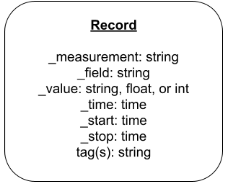
Anatomy of a Row
When read from the storage engine and passed into the filter function, by default, before being transformed by other functions, every row has the same essential object model. Flux uses a leading underscore (“_”) to delineate reserved member names. In Flux, each member of a row is called a “column,” or sometimes a “field” depending on the context.
We can see how this is generally represented as a row in Flux.
| _measurement | tag1 | _field | _value | _time |
| measurement1 | tagvalue1 | fieldname1 | 1.0 | rfc3339time1 |
r._measurementis a string that is the measurement which defines the table that row is saved into.r._fieldis a string that is the name of the field which defines the table that the row is saved into.r._valueis the actual value of the field.r._timeis the time stamp of the row.
Additionally, each tag value is accessible by its tag name. For example, r.tag1, which in this example has a value of “tagvalue1.”
Finally, there are two additional context specific members added. These members are determined by the query, not the underlying data:
r._startis the start time of the range() in the query.r._stop()is the stop time of the range() in the query.
For example, if you query with a range of 5 minutes in the past (range(start: -5m)), you will get a _start and _stop 5 minutes apart:
| _measurement | tag1 | _field | _value | _start | _stop | _time |
| measurement1 | tagvalue1 | fieldname1 | 1.0 | 2021:08:20T20:00:000000000Z | 2021:08:20T20:05:000000000Z | rfc3339time1 |
When you are filtering, you therefore have all of these columns to work from.
Filtering Measurements
A discussed in the data model section above, a measurement is the highest order aggregation of data inside a bucket. It is, therefore, the most common subject, and typically first, filter, as it filters out the most irrelevant data in a single statement.
Additionally, every table written by the storage engine has exactly one measurement, so the storage engine can quickly find the relevant tables and return them.
filter(fn: (r) => r._measurement == "measurement1")
Given the two tables below, only the first will be returned if the preceding filter is applied:
| _measurement | tag1 | _field | _value | _time |
| measurement1 | tagvalue1 | field1 | 1i | rfc3339time1 |
| measurement1 | tagvalue1 | field1 | 2i | rfc3339time2 |
| _measurement | tag1 | _field | _value | _time |
| measurement2 | tagvalue1 | field1 | 1.0 | rfc3339time1 |
| measurement2 | tagvalue1 | field1 | 2.0 | rfc3339time2 |
Filtering Tags
Multiple measurements can share the same tag set. As such, filtering by tag is sometimes secondary to filtering by measurement. The storage engine keeps track of where the tables with different tags for specific measurements are, so filtering by tag is typically reasonably fast.
The following tables have different measurements, but the same tag values, so the following filter will return both tables:
|> filter(fn: (r) => r.tag1 == "tagvalue1")
| _measurement | tag1 | _field | _value | _time |
| measurement1 | tagvalue1 | field1 | 1i | rfc3339time1 |
| measurement1 | tagvalue1 | field1 | 2i | rfc3339time2 |
| _measurement | tag1 | _field | _value | _time |
| measurement2 | tagvalue1 | field1 | 1.0 | rfc3339time1 |
| measurement2 | tagvalue1 | field1 | 2.0 | rfc3339time2 |
If you only want one measurement with that tag value, you can simply include both filters. The following will return only the first table:
|> filter(fn: (r) => r._measurement == "measurement1")
|> filter(fn: (r) => r.tag1 == "tagvalue1")
Filtering by Field
Filtering by field is extremely common, and also very fast, as fields are part of the group key of tables. Given the following table, if you are interested in records in field1 in measurement1, you can simply query like so, and get back only the first table:
|> filter(fn: (r) => r._field == "field1")
| _measurement | tag1 | _field | _value | _time |
| measurement1 | tagvalue1 | field1 | 1i | rfc3339time1 |
| measurement1 | tagvalue1 | field1 | 2i | rfc3339time2 |
| _measurement | tag1 | _field | _value | _time |
| measurement1 | tagvalue1 | field2 | 1.0 | rfc3339time1 |
| measurement1 | tagvalue1 | field2 | 2.0 | rfc3339time2 |
| _measurement | tag1 | _field | _value | _time |
| measurement2 | tagvalue1 | field2 | 3.0 | rfc3339time1 |
| measurement2 | tagvalue1 | field2 | 4.0 | rfc3339time2 |
However, this won’t work for field2, as that field name exists in measurement2 as well. Simply include a measurement filter as well:
|> filter(fn: (r) => r._measurement == "measurement1")
|> filter(fn: (r) => r._field == "field2")
This will return only the first table.
Filter by Exists
There may be circumstances where you wish to only operate on tables that contain a specific tag value. You can use exists or not exists for this.
The following will ensure that only tables which contain the “tag1” are returned:
|> filter(fn: (r) => exists r.tag1)
Similarly, if you want to retain only tables that do not conain the “tag1”, use:
|> filter(fn: (r) => not exists r.tag1)
To illustrate that point, take the following two tables. Each record has a different time stamp. The second table differs only in that those points were recorded with an additional tag, “tag2”.
| _measurement | tag1 | _field | _value | _time |
| measurement1 | tagvalue1 | field1 | 1i | rfc3339time3 |
| measurement1 | tagvalue1 | field1 | 2i | rfc3339time4 |
| _measurement | tag1 | tag2 | _field | _value | _time |
| measurement1 | tagvalue1 | tagvalue2 | field1 | 3i | rfc3339time1 |
| measurement1 | tagvalue1 | tagvalue2 | field1 | 4i | rfc3339time2 |
The following query will return the first table:
> filter(fn: (r) => not exists r.tag2) |
If you only wanted to return the second table with the points that lack the “tag2”, you can use not exists. Instead you must must drop that column all together. We’ll cover that in more detail in later sections.
Filtering by Field Value
Filtering by measurement(s), tag(s), or field(s) removes entire tables from the response. You can also filter out individual rows in tables. The most common way to do this is to filter by value.
For example, if we take our few rows of air sensor data, and first filter by field:
|> filter(fn: (r) => r._field == "fieldname1")
We are left with these two tables.
| _measurement | tag1 | _field | _value | _time |
| measurement1 | tagvalue1 | field1 | 1.0 | rfc3339time1 |
| measurement1 | tagvalue1 | field1 | 2.0 | rfc3339time2 |
| _measurement | tag1 | _field | _value | _time |
| measurement1 | tagvalue2 | field1 | 3.0 | rfc3339time1 |
| measurement1 | tagvalue2 | field1 | 3.0 | rfc3339time2 |
If we also add a filter for value, we can filter out individual rows. For example:
|> filter(fn: (r) => r._field == "field1")
|> filter(fn: (r) => r._value >= 2.0)
Will result in the following stream of tables being emitted:. Note that the first table has dropped a single row:
| _measurement | tag1 | _field | _value | _time |
| measurement1 | tagvalue1 | field1 | 2.0 | rfc3339time2 |
| _measurement | tag1 | _field | _value | _time |
| measurement1 | tagvalue2 | field1 | 3.0 | rfc3339time1 |
| measurement1 | tagvalue2 | field1 | 3.0 | rfc3339time2 |
The row where the field value was less than 2 was dropped.
Compound Filters
Boolean expressions in Flux can be compounded with “or” and “and.” For example, to retrieve all the tables with either the fields temperature or humidity, but no others, you use:
|> filter(fn: (r) => r._field == "field1" or r._field == "filed2")
You can aggregate with or using different members of r if needed:
|> filter(fn: (r) => r._field == "field1" or exist r.tag1)
You can use and as well:
|> filter(fn: (r) => r._field == "field1" and r.tag1 == "tagvalue1")
However, this is less commonly used because it is equivalent to simply supplying two filters. The follow two filters is equivalent to, and arguably easier to read and modify:
|> filter(fn: (r) => r._field == "field1")
|> filter(fn: (r) => r.sensor_id == "tagvalue1")
Regular Expressions
Sometimes your code will need to find substrings or even more complex pattern matching. Flux supports regular expressions for this purpose.
There are two regex operators in Flux, “=~” for matches, and “!~” for does not match. The operators expect a string on the left side, and regular expression on the right. You define a regular expression object by surrounding your regex in “/.” For example to find all values of tag1 that include the string “tag”. You can use:
|> filter(fn: (r) => r.tag1 =~ /tag/)
In this case, the regex operator is “matches”, i.e. find all of the tag1 values that match the regex, and the regex itself is tag. Every table where the tag1 tag value contains the string “tag” will be returned.
To exclude all such tables, simply use the “does not match” version:
|> filter(fn: (r) => r.tag1 !~ /tag/)
Flux supports the full range of regex expressiveness. To match the pattern of 3 capital letters and 4 digits:
|> filter(fn: (r) => r._value =~ /[A-Z]{3}[0-9]{4}/)
These operators work on any field that is of type string. So you can use this to filter by measurement, field name, and even field value when the field value is a string type.
However, it is important to note that the Flux storage engine cannot leverage the layout of tables when using regular expressions, so it must often scan every table, or even every row, to find matches. This can cause your queries to run much more slowly. Therefore, if you are regularly using regular expressions to filter your data, consider adding additional tags instead.
If, Then, Else
Flux also supports “if, then, else” statements. This can be useful if you want to express more complex conditions in a readable manner.
The following two filters are equivalent:
filter(fn: (r) => if r._value < 2.0 then true else  false)
filter(fn: (r) => r._value < 1.0)
Naturally, you can rather return the result of a boolean expression:
filter(fn: (r) => if r.tag1 == "tagvalue1" then r._value < 2.0 else false)
If then else can also be chained:
filter(fn: (r) => if r.tag1 == "tagvalue1"
then r._value < 2.0
else if r.tag1 == "tagvalue2"
	then r._value < 3.0
else false)
Types In Comparisons
As a strongly typed language, in general, Flux does not support comparisons between variables with different types.
Flux does support comparing integers to floats:
int( v: "1") == 1.0
But does not support comparing other data types. For example, this will cause an error:
"1" == 1.0
unsupported binary expression string == float
Times can be compared:
2021-07-12T19:38:00.000Z < 2021-07-12T19:39:00.000Z
But cannot be compared to, for example, Unix Time integers:
2021-07-12T19:38:00.000Z < 1627923626000000000
unsupported binary expression time < int
But this can be done with some explicit casting:
uint(v: 2021-07-12T19:38:00.000Z) < 1627923626000000000
Details on how to cast time between different formats so that you calculate and compare time and durations from different formats is covered in detail in a future section.
Queries and the Data Model
This section focused on queries that only found and filtered data. As such, the results are a subset of tables and a subset of rows of the tables stored in the storage engine. There may be few tables, but the only change to the tables returned is that there may be rows filtered out.
In other words, the pattern from() |> range() |> filter() will not transform your data as stored on disk other than perhaps filtering it. The next section will go further and delve into many of the options for transforming the shape of the data.
Flux Data Transformations
In addition to retrieving data from disk, Flux is a powerful data transformation tool. You can use Flux to shape your data however needed, as well as apply powerful mathematical transformations to your data as well.
Grouping
To review, when you write data to InfluxDB, the storage engine persists it in tables, where each table is defined by a “group key.” The group key used to persist the data is a measurement name, a unique set of tag values, and a field name.
Consider the following example of 12 tables with two rows each, all containing the same measurement, but there are:
- Two tags, with a total of 5 tag values
- tag1 has the 2 tag values:
- tagvalue1
- tagvalue4
- tag2 has 3 tag values:
- tagvalue2
- tagvalue3
- tagvalue5
- tag1 has the 2 tag values:
- Two fields
- field1
- field2
Where the line protocol would look like:
measurement,tag1=tagvalue1,tag2=tagvalue2 field1=0.0 unixtime1
measurement,tag1=tagvalue1,tag2=tagvalue2 field1=1.0 unixtime2

measurement,tag1=tagvalue4,tag2=tagvalue2 field1=0.0 unixtime1
measurement,tag1=tagvalue4,tag2=tagvalue2 field1=1.0 unixtime2

measurement,tag1=tagvalue1,tag2=tagvalue3 field1=0.0 unixtime1
measurement,tag1=tagvalue1,tag2=tagvalue3 field1=1.0 unixtime2

measurement,tag1=tagvalue4,tag2=tagvalue3 field1=0.0 unixtime1
measurement,tag1=tagvalue4,tag2=tagvalue3 field1=1.0 unixtime2

measurement,tag1=tagvalue1,tag2=tagvalue5 field1=0.0 unixtime1
measurement,tag1=tagvalue1,tag2=tagvalue5 field1=1.0 unixtime2

measurement,tag1=tagvalue4,tag2=tagvalue5 field1=0.0 unixtime1
measurement,tag1=tagvalue4,tag2=tagvalue5 field1=1.0 unixtime2

measurement,tag1=tagvalue1,tag2=tagvalue2 field2=0.0 unixtime1
measurement,tag1=tagvalue1,tag2=tagvalue2 field2=1.0 unixtime2

measurement,tag1=tagvalue4,tag2=tagvalue2 field2=0.0 unixtime1
measurement,tag1=tagvalue4,tag2=tagvalue2 field2=1.0 unixtime2

measurement,tag1=tagvalue1,tag2=tagvalue3 field2=0.0 unixtime1
measurement,tag1=tagvalue1,tag2=tagvalue3 field2=1.0 unixtime2

measurement,tag1=tagvalue4,tag2=tagvalue3 field2=0.0 unixtime1
measurement,tag1=tagvalue4,tag2=tagvalue3 field2=1.0 unixtime2

measurement,tag1=tagvalue1,tag2=tagvalue5 field2=0.0 unixtime1
measurement,tag1=tagvalue1,tag2=tagvalue5 field2=1.0 unixtime2

measurement,tag1=tagvalue4,tag2=tagvalue5 field2=0.0 unixtime1
measurement,tag1=tagvalue4,tag2=tagvalue5 field2=1.0 unixtime2
I encourage you to replace the metasyntax timestamps with actual unix timestamps and try out the grouping on your own. You can use can use this unix timestamp converter to get two unix timestamps of your choice or you can use the following two values:
1628229600000000000 (or 2021-08-06T06:00:00.000000000Z)1628229900000000000 (or 2021-08-06T06:05:00.000000000Z)
Then write the data to InfluxDB with the CLI, API, or InfluxDB UI.
The following query will return the following 12 separate tables:
from(bucket: "bucket1")
|> range(start: 0)
Note that an extra row has been added to each table to denote if each column is part of the group key. The start column has been removed from the table response for simplicity. The table column has been added to help you keep track of the number of columns. Remember, the group key for the table column is an exception and it’s always set to false. The group key for the table is set to false because users can’t directly change the table number. The table record will always be the same across rows even though the group key is set to false.
| Not in Group Key | In Group Key | In Group Key | In Group Key | In Group Key | Not in Group Key | Not in Group Key |
| table | _measurement | _field | tag1 | tag2 | _value | _time |
| 0 | measurement1 | field1 | tagvalue1 | tagvalue2 | 0.0 | rfc3339time1 |
| 0 | measurement1 | field1 | tagvalue1 | tagvalue2 | 1.0 | rfc3339time2 |
| Not in Group Key | In Group Key | In Group Key | In Group Key | In Group Key | Not in Group Key | Not in Group Key |
| table | _measurement | _field | tag1 | tag2 | _value | _time |
| 1 | measurement1 | field1 | tagvalue4 | tagvalue2 | 0.0 | rfc3339time1 |
| 1 | measurement1 | field1 | tagvalue4 | tagvalue2 | 1.0 | rfc3339time2 |
| Not in Group Key | In Group Key | In Group Key | In Group Key | In Group Key | Not in Group Key | Not in Group Key |
| table | _measurement | _field | tag1 | tag2 | _value | _time |
| 2 | measurement1 | field1 | tagvalue1 | tagvalue3 | 0.0 | rfc3339time1 |
| 2 | measurement1 | field1 | tagvalue1 | tagvalue3 | 1.0 | rfc3339time2 |
| Not in Group Key | In Group Key | In Group Key | In Group Key | In Group Key | Not in Group Key | Not in Group Key |
| table | _measurement | _field | tag1 | tag2 | _value | _time |
| 3 | measurement1 | field1 | tagvalue4 | tagvalue3 | 0.0 | rfc3339time1 |
| 3 | measurement1 | field1 | tagvalue4 | tagvalue3 | 1.0 | rfc3339time2 |
| Not in Group Key | In Group Key | In Group Key | In Group Key | In Group Key | Not in Group Key | Not in Group Key |
| table | _measurement | _field | tag1 | tag2 | _value | _time |
| 4 | measurement1 | field1 | tagvalue1 | tagvalue5 | 0.0 | rfc3339time1 |
| 4 | measurement1 | field1 | tagvalue1 | tagvalue5 | 1.0 | rfc3339time2 |
| Not in Group Key | In Group Key | In Group Key | In Group Key | In Group Key | Not in Group Key | Not in Group Key |
| table | _measurement | _field | tag1 | tag2 | _value | _time |
| 5 | measurement1 | field1 | tagvalue4 | tagvalue5 | 0.0 | rfc3339time1 |
| 5 | measurement1 | field1 | tagvalue4 | tagvalue5 | 1.0 | rfc3339time2 |
Aaa
| Not in Group Key | In Group Key | In Group Key | In Group Key | In Group Key | Not in Group Key | Not in Group Key |
| table | _measurement | _field | tag1 | tag2 | _value | _time |
| 6 | measurement1 | field2 | tagvalue1 | tagvalue2 | 0.0 | rfc3339time1 |
| 6 | measurement1 | field2 | tagvalue1 | tagvalue2 | 1.0 | rfc3339time2 |
| Not in Group Key | In Group Key | In Group Key | In Group Key | In Group Key | Not in Group Key | Not in Group Key |
| table | _measurement | _field | tag1 | tag2 | _value | _time |
| 7 | measurement1 | field2 | tagvalue4 | tagvalue2 | 0.0 | rfc3339time1 |
| 7 | measurement1 | field2 | tagvalue4 | tagvalue2 | 1.0 | rfc3339time2 |
| Not in Group Key | In Group Key | In Group Key | In Group Key | In Group Key | Not in Group Key | Not in Group Key |
| table | _measurement | _field | tag1 | tag2 | _value | _time |
| 8 | measurement1 | field2 | tagvalue1 | tagvalue3 | 0.0 | rfc3339time1 |
| 8 | measurement1 | field2 | tagvalue1 | tagvalue3 | 1.0 | rfc3339time2 |
| Not in Group Key | In Group Key | In Group Key | In Group Key | In Group Key | Not in Group Key | Not in Group Key |
| table | _measurement | _field | tag1 | tag2 | _value | _time |
| 9 | measurement1 | field2 | tagvalue4 | tagvalue3 | 0.0 | rfc3339time1 |
| 9 | measurement1 | field2 | tagvalue4 | tagvalue3 | 1.0 | rfc3339time2 |
| Not in Group Key | In Group Key | In Group Key | In Group Key | In Group Key | Not in Group Key | Not in Group Key |
| table | _measurement | _field | tag1 | tag2 | _value | _time |
| 10 | measurement1 | field2 | tagvalue1 | tagvalue5 | 0.0 | rfc3339time1 |
| 10 | measurement1 | field2 | tagvalue1 | tagvalue5 | 1.0 | rfc3339time2 |
| Not in Group Key | In Group Key | In Group Key | In Group Key | In Group Key | Not in Group Key | Not in Group Key |
| table | _measurement | _field | tag1 | tag2 | _value | _time |
| 11 | measurement1 | field2 | tagvalue4 | tagvalue5 | 0.0 | rfc3339time1 |
| 11 | measurement1 | field2 | tagvalue4 | tagvalue5 | 1.0 | rfc3339time2 |
By default each field name will be in a separate table, and then there are 6 unique combinations of tag values grouped with each field:
- tagvalue1 and tagvalue2
- tagvalue4 and tagvalue2
- tagvalue1 and tagvalue3
- tagvalue4 and tagvalue3
- tagvalue1 and tagvalue5
- tagvalue4 and tagvalue5
group()
The group() function can be to redefine the group keys, which will then result in regrouping the tables. We can begin by examining how defined the group key to a single column can affect the tables.
from(bucket: "bucket1")
|> range(start: 0)
|> group(columns: ["tag1"])
We know that there are 2 tag values for tag1 (tagvalue1 and tagvalue4), so we can predict that there will be two tables after the grouping:
| Not In Group Key | Not In Group Key | Not In Group Key | In Group Key | Not in Group Key | Not in Group Key | Not in Group Key |
| table | _measurement | _field | tag1 | tag2 | _value | _time |
| 0 | measurement1 | field1 | tagvalue1 | tagvalue2 | 0.0 | rfc3339time1 |
| 0 | measurement1 | field1 | tagvalue1 | tagvalue2 | 1.0 | rfc3339time2 |
| 0 | measurement1 | field1 | tagvalue1 | tagvalue3 | 0.0 | rfc3339time1 |
| 0 | measurement1 | field1 | tagvalue1 | tagvalue3 | 1.0 | rfc3339time2 |
| 0 | measurement1 | field1 | tagvalue1 | tagvalue5 | 0.0 | rfc3339time1 |
| 0 | measurement1 | field1 | tagvalue1 | tagvalue5 | 1.0 | rfc3339time2 |
| 0 | measurement1 | field2 | tagvalue1 | tagvalue2 | 0.0 | rfc3339time1 |
| 0 | measurement1 | field2 | tagvalue1 | tagvalue2 | 1.0 | rfc3339time2 |
| 0 | measurement1 | field2 | tagvalue1 | tagvalue3 | 0.0 | rfc3339time1 |
| 0 | measurement1 | field2 | tagvalue1 | tagvalue3 | 1.0 | rfc3339time2 |
| 0 | measurement1 | field2 | tagvalue1 | tagvalue5 | 0.0 | rfc3339time1 |
| 0 | measurement1 | field2 | tagvalue1 | tagvalue5 | 1.0 | rfc3339time2 |
| Not In Group Key | Not In Group Key | Not In Group Key | In Group Key | Not in Group Key | Not in Group Key | Not in Group Key |
| table | _measurement | _field | tag1 | tag2 | _value | _time |
| 1 | measurement1 | field1 | tagvalue4 | tagvalue2 | 0.0 | rfc3339time1 |
| 1 | measurement1 | field1 | tagvalue4 | tagvalue2 | 1.0 | rfc3339time2 |
| 1 | measurement1 | field1 | tagvalue4 | tagvalue3 | 0.0 | rfc3339time1 |
| 1 | measurement1 | field1 | tagvalue4 | tagvalue3 | 1.0 | rfc3339time2 |
| 1 | measurement1 | field1 | tagvalue4 | tagvalue5 | 0.0 | rfc3339time1 |
| 1 | measurement1 | field1 | tagvalue4 | tagvalue5 | 1.0 | rfc3339time2 |
| 1 | measurement1 | field2 | tagvalue4 | tagvalue2 | 0.0 | rfc3339time1 |
| 1 | measurement1 | field2 | tagvalue4 | tagvalue2 | 1.0 | rfc3339time2 |
| 1 | measurement1 | field2 | tagvalue4 | tagvalue3 | 0.0 | rfc3339time1 |
| 1 | measurement1 | field2 | tagvalue4 | tagvalue3 | 1.0 | rfc3339time2 |
| 1 | measurement1 | field2 | tagvalue4 | tagvalue5 | 0.0 | rfc3339time1 |
| 1 | measurement1 | field2 | tagvalue4 | tagvalue5 | 1.0 | rfc3339time2 |
If we group by both tags, then we can predict that there will be 6 tables because, as described above, there are three unique combinations of tag values:
from(bucket: "bucket1")
|> range(start: 0)
|> group(columns: ["tag1", "tag2"])
| Not In Group Key | Not In Group Key | In Group Key | In Group Key | Not In Group Key | Not in Group Key | Not in Group Key |
| table | _measurement | _field | tag1 | tag2 | _value | _time |
| 0 | measurement1 | field1 | tagvalue1 | tagvalue2 | 0.0 | rfc3339time1 |
| 0 | measurement1 | field1 | tagvalue1 | tagvalue2 | 1.0 | rfc3339time2 |
| 0 | measurement1 | field2 | tagvalue1 | tagvalue2 | 0.0 | rfc3339time1 |
| 0 | measurement1 | field2 | tagvalue1 | tagvalue2 | 1.0 | rfc3339time2 |
| Not In Group Key | Not In Group Key | In Group Key | In Group Key | Not In Group Key | Not in Group Key | Not in Group Key |
| table | _measurement | _field | tag1 | tag2 | _value | _time |
| 1 | measurement1 | field1 | tagvalue4 | tagvalue2 | 0.0 | rfc3339time1 |
| 1 | measurement1 | field1 | tagvalue4 | tagvalue2 | 1.0 | rfc3339time2 |
| 1 | measurement1 | field2 | tagvalue4 | tagvalue2 | 0.0 | rfc3339time1 |
| 1 | measurement1 | field2 | tagvalue4 | tagvalue2 | 1.0 | rfc3339time2 |
| Not In Group Key | Not In Group Key | In Group Key | In Group Key | Not In Group Key | Not in Group Key | Not in Group Key |
| table | _measurement | _field | tag1 | tag2 | _value | _time |
| 2 | measurement1 | field1 | tagvalue1 | tagvalue3 | 0.0 | rfc3339time1 |
| 2 | measurement1 | field1 | tagvalue1 | tagvalue3 | 1.0 | rfc3339time2 |
| 2 | measurement1 | field2 | tagvalue1 | tagvalue3 | 0.0 | rfc3339time1 |
| 2 | measurement1 | field2 | tagvalue1 | tagvalue3 | 1.0 | rfc3339time2 |
| Not In Group Key | Not In Group Key | In Group Key | In Group Key | Not In Group Key | Not in Group Key | Not in Group Key |
| table | _measurement | _field | tag1 | tag2 | _value | _time |
| 3 | measurement1 | field1 | tagvalue4 | tagvalue3 | 0.0 | rfc3339time1 |
| 3 | measurement1 | field1 | tagvalue4 | tagvalue3 | 1.0 | rfc3339time2 |
| 3 | measurement1 | field2 | tagvalue4 | tagvalue3 | 0.0 | rfc3339time1 |
| 3 | measurement1 | field2 | tagvalue4 | tagvalue3 | 1.0 | rfc3339time2 |
| Not In Group Key | Not In Group Key | In Group Key | In Group Key | Not In Group Key | Not in Group Key | Not in Group Key |
| table | _measurement | _field | tag1 | tag2 | _value | _time |
| 4 | measurement1 | field1 | tagvalue1 | tagvalue5 | 0.0 | rfc3339time1 |
| 4 | measurement1 | field1 | tagvalue1 | tagvalue5 | 1.0 | rfc3339time2 |
| 4 | measurement1 | field2 | tagvalue1 | tagvalue5 | 0.0 | rfc3339time1 |
| 4 | measurement1 | field2 | tagvalue1 | tagvalue5 | 1.0 | rfc3339time2 |
| Not In Group Key | Not In Group Key | In Group Key | In Group Key | Not In Group Key | Not in Group Key | Not in Group Key |
| table | _measurement | _field | tag1 | tag2 | _value | _time |
| 5 | measurement1 | field1 | tagvalue4 | tagvalue5 | 0.0 | rfc3339time1 |
| 5 | measurement1 | field1 | tagvalue4 | tagvalue5 | 1.0 | rfc3339time2 |
| 5 | measurement1 | field2 | tagvalue4 | tagvalue5 | 0.0 | rfc3339time1 |
| 5 | measurement1 | field2 | tagvalue4 | tagvalue5 | 1.0 | rfc3339time2 |
Grouping by field alone, we can predict that we will see a total of 2 tables, because the data set has only 2 field names.
from(bucket: "bucket1")
|> range(start: 0)
|> group(columns: ["_field"])
| Not In Group Key | Not In Group Key | In Group Key | Not In Group Key | Not In Group Key | Not in Group Key | Not in Group Key |
| table | _measurement | _field | tag1 | tag2 | _value | _time |
| 0 | measurement1 | field1 | tagvalue1 | tagvalue2 | 0.0 | rfc3339time1 |
| 0 | measurement1 | field1 | tagvalue1 | tagvalue2 | 1.0 | rfc3339time2 |
| 0 | measurement1 | field1 | tagvalue4 | tagvalue2 | 0.0 | rfc3339time1 |
| 0 | measurement1 | field1 | tagvalue4 | tagvalue2 | 1.0 | rfc3339time2 |
| 0 | measurement1 | field1 | tagvalue1 | tagvalue3 | 0.0 | rfc3339time1 |
| 0 | measurement1 | field1 | tagvalue1 | tagvalue3 | 1.0 | rfc3339time2 |
| 0 | measurement1 | field1 | tagvalue4 | tagvalue3 | 0.0 | rfc3339time1 |
| 0 | measurement1 | field1 | tagvalue4 | tagvalue3 | 1.0 | rfc3339time2 |
| 0 | measurement1 | field1 | tagvalue1 | tagvalue5 | 0.0 | rfc3339time1 |
| 0 | measurement1 | field1 | tagvalue1 | tagvalue5 | 1.0 | rfc3339time2 |
| 0 | measurement1 | field1 | tagvalue4 | tagvalue5 | 0.0 | rfc3339time1 |
| 0 | measurement1 | field1 | tagvalue4 | tagvalue5 | 1.0 | rfc3339time2 |
| Not In Group Key | Not In Group Key | In Group Key | Not In Group Key | Not In Group Key | Not in Group Key | Not in Group Key |
| table | _measurement | _field | tag1 | tag2 | _value | _time |
| 1 | measurement1 | field2 | tagvalue1 | tagvalue2 | 0.0 | rfc3339time1 |
| 1 | measurement1 | field2 | tagvalue1 | tagvalue2 | 1.0 | rfc3339time2 |
| 1 | measurement1 | field2 | tagvalue4 | tagvalue2 | 0.0 | rfc3339time1 |
| 1 | measurement1 | field2 | tagvalue4 | tagvalue2 | 1.0 | rfc3339time2 |
| 1 | measurement1 | field2 | tagvalue1 | tagvalue3 | 0.0 | rfc3339time1 |
| 1 | measurement1 | field2 | tagvalue1 | tagvalue3 | 1.0 | rfc3339time2 |
| 1 | measurement1 | field2 | tagvalue4 | tagvalue3 | 0.0 | rfc3339time1 |
| 1 | measurement1 | field2 | tagvalue4 | tagvalue3 | 1.0 | rfc3339time2 |
| 1 | measurement1 | field2 | tagvalue1 | tagvalue5 | 0.0 | rfc3339time1 |
| 1 | measurement1 | field2 | tagvalue1 | tagvalue5 | 1.0 | rfc3339time2 |
| 1 | measurement1 | field2 | tagvalue4 | tagvalue5 | 0.0 | rfc3339time1 |
| 1 | measurement1 | field2 | tagvalue4 | tagvalue5 | 1.0 | rfc3339time2 |
Any combination of columns can be used for grouping depending on your purposes. For example, we can ask for tables for each field with each value for tag1. We can predict that there will be 4 such tables, because there are two fields and two tag values for tag1:
from(bucket: "bucket1")
|> range(start: 0)
|> group(columns: ["_field", "tag1"])
| Not In Group Key | Not In Group Key | In Group Key | In Group Key | Not In Group Key | Not in Group Key | Not in Group Key |
| table | _measurement | _field | tag1 | tag2 | _value | _time |
| 0 | measurement1 | field1 | tagvalue1 | tagvalue2 | 0.0 | rfc3339time1 |
| 0 | measurement1 | field1 | tagvalue1 | tagvalue2 | 1.0 | rfc3339time2 |
| 0 | measurement1 | field1 | tagvalue1 | tagvalue3 | 0.0 | rfc3339time1 |
| 0 | measurement1 | field1 | tagvalue1 | tagvalue3 | 1.0 | rfc3339time2 |
| 0 | measurement1 | field1 | tagvalue1 | tagvalue5 | 0.0 | rfc3339time1 |
| 0 | measurement1 | field1 | tagvalue1 | tagvalue5 | 1.0 | rfc3339time2 |
| Not In Group Key | Not In Group Key | In Group Key | In Group Key | Not In Group Key | Not in Group Key | Not in Group Key |
| table | _measurement | _field | tag1 | tag2 | _value | _time |
| 1 | measurement1 | field1 | tagvalue4 | tagvalue2 | 0.0 | rfc3339time1 |
| 1 | measurement1 | field1 | tagvalue4 | tagvalue2 | 1.0 | rfc3339time2 |
| 1 | measurement1 | field1 | tagvalue4 | tagvalue3 | 0.0 | rfc3339time1 |
| 1 | measurement1 | field1 | tagvalue4 | tagvalue3 | 1.0 | rfc3339time2 |
| 1 | measurement1 | field1 | tagvalue4 | tagvalue5 | 0.0 | rfc3339time1 |
| 1 | measurement1 | field1 | tagvalue4 | tagvalue5 | 1.0 | rfc3339time2 |
| Not In Group Key | Not In Group Key | In Group Key | In Group Key | Not In Group Key | Not in Group Key | Not in Group Key |
| table | _measurement | _field | tag1 | tag2 | _value | _time |
| 2 | measurement1 | field2 | tagvalue1 | tagvalue2 | 0.0 | rfc3339time1 |
| 2 | measurement1 | field2 | tagvalue1 | tagvalue2 | 1.0 | rfc3339time2 |
| 2 | measurement1 | field2 | tagvalue1 | tagvalue3 | 0.0 | rfc3339time1 |
| 2 | measurement1 | field2 | tagvalue1 | tagvalue3 | 1.0 | rfc3339time2 |
| 2 | measurement1 | field2 | tagvalue1 | tagvalue5 | 0.0 | rfc3339time1 |
| 2 | measurement1 | field2 | tagvalue1 | tagvalue5 | 1.0 | rfc3339time2 |
| Not In Group Key | Not In Group Key | In Group Key | In Group Key | Not In Group Key | Not in Group Key | Not in Group Key |
| table | _measurement | _field | tag1 | tag2 | _value | _time |
| 3 | measurement1 | field2 | tagvalue4 | tagvalue2 | 0.0 | rfc3339time1 |
| 3 | measurement1 | field2 | tagvalue4 | tagvalue2 | 1.0 | rfc3339time2 |
| 3 | measurement1 | field2 | tagvalue4 | tagvalue3 | 0.0 | rfc3339time1 |
| 3 | measurement1 | field2 | tagvalue4 | tagvalue3 | 1.0 | rfc3339time2 |
| 3 | measurement1 | field2 | tagvalue4 | tagvalue5 | 0.0 | rfc3339time1 |
| 3 | measurement1 | field2 | tagvalue4 | tagvalue5 | 1.0 | rfc3339time2 |
group() and Type Conflicts
In the above example, the values for field1 and field2 were always floats. Therefore, when grouping both of those fields into the same tables, it worked. However, recall that a column in InfluxDB can only have one type.
Given the following two tables which differ only in that they have a different field name, and their field values have a different type:
| table | _measurement | _field | _value | _time |
| 0 | measurement1 | field1 | 1i | rfc3339time2 |
| table | _measurement | _field | _value | _time |
| 1 | measurement1 | field2 | 1.0 | rfc3339time2 |
An attempt to group these two tables into the same table will result in the following error:
from(bucket: "bucket1")
|> range(start: 0)
|> group()
schema collision: cannot group integer and float types together
The simplest way to address this is to convert all of the values to floats using the toFloat() function. This function simply converts the value field for each record into a float if possible.
from(bucket: "bucket1")
|> range(start: 0)
|> toFloat()
|> group()
| table | _measurement | _field | _value | _time |
| 0 | measurement1 | field1 | 1.0 | rfc3339time2 |
| 0 | measurement1 | field2 | 1.0 | rfc3339time2 |
drop()/keep()
Another way to affect the group keys is to simply remove columns that are in the group key using the drop() or keep() functions. These two functions operate in the same manner, it’s just a matter of supplying a list of columns to eliminate vs. preserve.
Note that the following are equivalent:
from(bucket: "bucket1")
|> range(start: 0)
|> drop(columns: ["tag1","tag2"])

from(bucket: "bucket1")
|> range(start: 0)
|> keep(columns: ["_measurement","_field","_value","_time"])
In both cases the effect is to remove both of the tag columns from the table. Because tags are always in the group key by default, this change will leave only _measurement and _field in the group key. Because there is only one measurement, this will result in grouping solely by _field.
| Not in Group Key | In Group Key | In Group Key | Not in Group Key | Not in Group Key |
| table | _measurement | _field | _value | _time |
| 0 | measurement1 | field1 | 0.0 | 2021-08-17T21:22:00.000000000Z |
| 0 | measurement1 | field1 | 1.0 | 2021-08-17T21:22:01.000000000Z |
| 0 | measurement1 | field1 | 0.0 | 2021-08-17T21:22:02.000000000Z |
| 0 | measurement1 | field1 | 1.0 | 2021-08-17T21:22:03.000000000Z |
| 0 | measurement1 | field1 | 0.0 | 2021-08-17T21:22:04.000000000Z |
| 0 | measurement1 | field1 | 1.0 | 2021-08-17T21:22:05.000000000Z |
| Not in Group Key | In Group Key | In Group Key | Not in Group Key | Not in Group Key |
| 1 | _measurement | _field | _value | _time |
| 1 | measurement1 | field1 | 0.0 | 2021-08-17T21:22:00.000000000Z |
| 1 | measurement1 | field1 | 1.0 | 2021-08-17T21:22:01.000000000Z |
| 1 | measurement1 | field1 | 0.0 | 2021-08-17T21:22:02.000000000Z |
| 1 | measurement1 | field1 | 1.0 | 2021-08-17T21:22:03.000000000Z |
| 1 | measurement1 | field1 | 0.0 | 2021-08-17T21:22:04.000000000Z |
| 1 | measurement1 | field1 | 1.0 | 2021-08-17T21:22:05.000000000Z |
Note that drop() and keep() are both susceptible to the same type conflicts that can cause errors with group().
rename()
The rename() function does not change the group key, but simply changes the names of the columns. It works by providing the function with a mapping of old column names to new column names.
Given the following very simple table:
| _measurement | tag1 | _field | _value | _time |
| measurement1 | tagvalue1 | field1 | 1i | rfc3339time1 |
The following code simply renames the tag1 column:
from(bucket: "bucket1")
|> range(start: 0)
|> rename(columns: {"tag1":"tag2"})
| _measurement | tag2 | _field | _value | _time |
| measurement1 | tagvalue1 | field1 | 1i | rfc3339time1 |
You can rename any column which can be very useful for things like formatting data to present to users. However, renaming can have some unintended consequences. For example, if you rename the _value column, certain functions will have surprising results or fail because they operate on _value.
from(bucket: "bucket1")
|> range(start: 0)
|> rename(columns: {"_value":"astring"})
| _measurement | tag1 | _field | astring | _time |
| measurement1 | tagvalue1 | field1 | 1i | rfc3339time1 |
from(bucket: "bucket1")
|> range(start: 0)
|> rename(columns: {"_value":"astring"})
|> toFloat()
| _measurement | tag1 | _field | _value | astring | _time |
| measurement1 | tagvalue1 | field1 | 1i | rfc3339time1 |
In this case, because there was no _value column to convert from, the toFloat() method had no data to place in the _value column that it creates.
Creating a Single Table or Ungrouping
Finally, it is possible to put all of the data into a single table assuming that you avoid type conflicts. This is achieved by using the group() function with no arguments. Basically making the group key empty, so all of the data gets grouped into a single table. This is effectively the same as ungrouping.
from(bucket: "bucket1")
  |> range(start: 0)
  |> group()
| Not In Group Key | Not In Group Key | In Group Key | Not In Group Key | Not In Group Key | Not in Group Key | Not in Group Key |
| table | _measurement | _field | tag1 | tag2 | _value | _time |
| 0 | measurement1 | field1 | tagvalue1 | tagvalue2 | 0.0 | rfc3339time1 |
| 0 | measurement1 | field1 | tagvalue1 | tagvalue2 | 1.0 | rfc3339time2 |
| 0 | measurement1 | field1 | tagvalue4 | tagvalue2 | 0.0 | rfc3339time1 |
| 0 | measurement1 | field1 | tagvalue4 | tagvalue2 | 1.0 | rfc3339time2 |
| 0 | measurement1 | field1 | tagvalue1 | tagvalue3 | 0.0 | rfc3339time1 |
| 0 | measurement1 | field1 | tagvalue1 | tagvalue3 | 1.0 | rfc3339time2 |
| 0 | measurement1 | field1 | tagvalue4 | tagvalue3 | 0.0 | rfc3339time1 |
| 0 | measurement1 | field1 | tagvalue4 | tagvalue3 | 1.0 | rfc3339time2 |
| 0 | measurement1 | field1 | tagvalue1 | tagvalue5 | 0.0 | rfc3339time1 |
| 0 | measurement1 | field1 | tagvalue1 | tagvalue5 | 1.0 | rfc3339time2 |
| 0 | measurement1 | field1 | tagvalue4 | tagvalue5 | 0.0 | rfc3339time1 |
| 0 | measurement1 | field1 | tagvalue4 | tagvalue5 | 1.0 | rfc3339time2 |
| 0 | measurement1 | field2 | tagvalue1 | tagvalue2 | 0.0 | rfc3339time1 |
| 0 | measurement1 | field2 | tagvalue1 | tagvalue2 | 1.0 | rfc3339time2 |
| 0 | measurement1 | field2 | tagvalue4 | tagvalue2 | 0.0 | rfc3339time1 |
| 0 | measurement1 | field2 | tagvalue4 | tagvalue2 | 1.0 | rfc3339time2 |
| 0 | measurement1 | field2 | tagvalue1 | tagvalue3 | 0.0 | rfc3339time1 |
| 0 | measurement1 | field2 | tagvalue1 | tagvalue3 | 1.0 | rfc3339time2 |
| 0 | measurement1 | field2 | tagvalue4 | tagvalue3 | 0.0 | rfc3339time1 |
| 0 | measurement1 | field2 | tagvalue4 | tagvalue3 | 1.0 | rfc3339time2 |
| 0 | measurement1 | field2 | tagvalue1 | tagvalue5 | 0.0 | rfc3339time1 |
| 0 | measurement1 | field2 | tagvalue1 | tagvalue5 | 1.0 | rfc3339time2 |
| 0 | measurement1 | field2 | tagvalue4 | tagvalue5 | 0.0 | rfc3339time1 |
| 0 | measurement1 | field2 | tagvalue4 | tagvalue5 | 1.0 | rfc3339time2 |
Windowing
Windowing is when you group data by the start and stop times with the window() function. In previous sections the _start and _stop columns have been omitted for simplicity because they usually represent the start and stop times defined in the range function and their values remain unchanged. However, the window() function affects the values of the _start and _stop columns so we’ll include these columns in this section. The window() function doesn’t affect the _time column, so we’ll exclude this column to simplify the examples in this section. To illustrate how the window() function works let’s filter our data for tagvalue1 and tagvalue4 and include the _start and _stop columns:
from(bucket: "bucket1")
  |> range(start: 2021-08-17T00:00:00, stop:2021-08-17T3:00:00 )
  |> filter(fn: (r) => r["tag1"] == "tagvalue1" or r["tag1"] == "tagvalue4")
  |> filter(fn: (r) => r["_field"] == "field1")
| Not in Group Key | In Group Key | In Group Key | In Group Key | In Group Key | In Group Key | In Group Key | Not in Group Key | Not in Group Key |
| table | _start | _stop | _measurement | _field | tag1 | tag2 | _value | _time |
| 0 | 2021-08-17T00:00:00 | 2021-08-17T03:00:00 | measurement1 | field1 | tagvalue1 | tagvalue2 | 0.0 | 2021-08-17T01:00:00 |
| 0 | 2021-08-17T00:00:00 | 2021-08-17T03:00:00 | measurement1 | field1 | tagvalue1 | tagvalue2 | 1.0 | 2021-08-17T02:00:00 |
| Not in Group Key | In Group Key | In Group Key | In Group Key | In Group Key | In Group Key | In Group Key | Not in Group Key | Not in Group Key |
| table | _start | _stop | _measurement | _field | tag1 | tag2 | _value | _time |
| 1 | 2021-08-17T00:00:00 | 2021-08-17T03:00:00 | measurement1 | field1 | tagvalue4 | tagvalue2 | 0.0 | 2021-08-17T01:00:00 |
| 1 | 2021-08-17T00:00:00 | 2021-08-17T03:00:00 | measurement1 | field1 | tagvalue4 | tagvalue2 | 1.0 | 2021-08-17T02:00:00 |
If you apply the window() function the values in the _start and _stop column will change to reflect the defined window period:
from(bucket: "bucket1")
  |> range(start: 2021-08-17T00:00:00, stop:2021-08-17T3:00:00 )
  |> filter(fn: (r) => r["tag1"] == "tagvalue1" or r["tag1"] == "tagvalue4")
  |> filter(fn: (r) => r["tag2"] == "tagvalue2")
  |> window(period: 90m)
  // the following syntax is synonymous with the line above |> window(every: 90m)
| Not in Group Key | In Group Key | In Group Key | In Group Key | In Group Key | In Group Key | In Group Key | Not in Group Key | Not in Group Key |
| table | _start | _stop | _measurement | _field | tag1 | tag2 | _value | _time |
| 0 | 2021-08-17T00:00:00 | 2021-08-17T01:30:00 | measurement1 | field1 | tagvalue1 | tagvalue2 | 0.0 | 2021-08-17T01:00:00 |
| Not in Group Key | In Group Key | In Group Key | In Group Key | In Group Key | In Group Key | In Group Key | Not in Group Key | Not in Group Key |
| table | _start | _stop | _measurement | _field | tag1 | tag2 | _value | _time |
| 1 | 2021-08-17T00:00:00 | 2021-08-17T01:30:00 | measurement1 | field1 | tagvalue4 | tagvalue2 | 0.0 | 2021-08-17T01:00:00 |
| Not in Group Key | In Group Key | In Group Key | In Group Key | In Group Key | In Group Key | In Group Key | Not in Group Key | Not in Group Key |
| table | _start | _stop | _measurement | _field | tag1 | tag2 | _value | _time |
| 2 | 2021-08-17T01:30:00 | 2021-08-17T03:00:00 | measurement1 | field1 | tagvalue1 | tagvalue2 | 1.0 | 2021-08-17T02:00:00 |
| Not in Group Key | In Group Key | In Group Key | In Group Key | In Group Key | In Group Key | In Group Key | Not in Group Key | Not in Group Key |
| table | _start | _stop | _measurement | _field | tag1 | tag2 | _value | _time |
| 3 | 2021-08-17T01:30:00 | 2021-08-17T03:00:00 | measurement1 | field1 | tagvalue4 | tagvalue2 | 1.0 | 2021-08-17T02:00:00 |
The boundary for the window period, as defined by either the period or every paramenter, is not based on execution time or the timestamps of any points returned by the range function. Instead windowing occurs at the top of the second, minute, hour, month, year. Additionally, The window boundaries or groupings won’t exceed the timestamps of the data you return from the range function. For example, imagine the following scenario: You query for data with |> range(start: 2022-01-20T20:18:00.000Z, stop: 2022-01-20T21:19:25.000Z) and your last record has a timestamp in that range of 2022-01-20T20:19:20.000Z. You’re every/periodduration is 30s. Then your last window group will have a _start value of 2022-01-20T20:19:00.000Z and a _stop of value of 2022-01-20T20:19:30.000Z. Notice how window grouping does not extend until the stop value specified by the range function. Instead, the grouping stops to include the final point.
Windowing is performed for two main reasons:
- To aggregate data across fields or tags with timestamps in the same period.
- To transform high precision series into a lower resolution aggregation.
To aggregate data across fields or tags with similar timestamps, you can first apply the window() function like above, then you can group your data by the _start times. Now data that’s in the same window will be in the same table, so you can apply an aggregation after:
from(bucket: "bucket1")
  |> range(start: 2021-08-17T00:00:00, stop:2021-08-17T3:00:00 )
  |> filter(fn: (r) => r["tag1"] == "tagvalue1" or r["tag1"] == "tagvalue4")
  |> window(period: 90m)
  |> group(columns: ["_start"], mode:"by")
  |> yield(name:"after group")
  |> sum()
  |> yield(name:"after sum")
The result after the first yield, “after group” looks like:
| Not in Group Key | In Group Key | In Group Key | In Group Key | In Group Key | Not in Group Key | Not in Group Key | Not in Group Key | Not in Group Key |
| table | _start | _stop | _measurement | _field | tag1 | tag2 | _value | _time |
| 0 | 2021-08-17T00:00:00 | 2021-08-17T01:30:00 | measurement1 | field1 | tagvalue1 | tagvalue2 | 0.0 | 2021-08-17T01:00:00 |
| 0 | 2021-08-17T00:00:00 | 2021-08-17T01:30:00 | measurement1 | field1 | tagvalue4 | tagvalue2 | 0.0 | 2021-08-17T01:00:00 |
| Not in Group Key | In Group Key | In Group Key | In Group Key | In Group Key | In Group Key | In Group Key | Not in Group Key | Not in Group Key |
| table | _start | _stop | _measurement | _field | tag1 | tag2 | _value | _time |
| 1 | 2021-08-17T01:30:00 | 2021-08-17T03:00:00 | measurement1 | field1 | tagvalue1 | tagvalue2 | 1.0 | 2021-08-17T02:00:00 |
| 1 | 2021-08-17T01:30:00 | 2021-08-17T03:00:00 | measurement1 | field1 | tagvalue4 | tagvalue2 | 1.0 | 2021-08-17T02:00:00 |
The result after the first yield, “after sum” looks like:
| Not in Group Key | In Group Key | In Group Key | In Group Key | In Group Key | Not in Group Key | Not in Group Key | Not in Group Key |
| table | _start | _stop | _measurement | _field | tag1 | tag2 | _value |
| 0 | 2021-08-17T00:00:00 | 2021-08-17T01:30:00 | measurement1 | field1 | tagvalue1 | tagvalue2 | 0.0 |
| Not in Group Key | In Group Key | In Group Key | In Group Key | In Group Key | In Group Key | In Group Key | Not in Group Key |
| table | _start | _stop | _measurement | _field | tag1 | tag2 | _value |
| 1 | 2021-08-17T01:30:00 | 2021-08-17T03:00:00 | measurement1 | field1 | tagvalue1 | tagvalue2 | 2.0 |
The sum() function is an aggregator so the _time column is removed because there isn’t a timestamp associated with the sum of two values. Keep in mind that in this example the timestamps in the _time column in the “after group” output happen to be the same, but this aggregation across fields within time windows would work even if the timestamps were different. The _time column isn’t a part of the group key.
Windowing back in time
When you apply the window() function, you group data on forward in time or create window bounds that align with the start of your data. You can’t window back it time, but you can produce the same effect by using the offset parameter. This parameter specifies the duration to shift the window boundaries by. You can use the offset parameter to make the windows always align with the current time which effectively groups the data backwards in time.
option offset = duration(v: int(v: now()))

data = from(bucket: "bucket1")
  |> range(start: -1m)
  |> filter(fn: (r) => r["_measurement"] == "measurement1")
  |> yield(name: "data")

data
  |> aggregateWindow(every: 30s, fn: mean, createEmpty: false, offset: offset)
  |> yield(name: "offset effectively windowing backward in time")
Alternatively, you could calculate the duration difference between your actual start time and the required start time so that your windows align with stop time instead. Then you could add that duration to the start with the offset parameter. The previous approach is the recommended approach, but examining multiple approaches lends us an appreciation for the power and flexibility that Flux provides.
data = from(bucket: "bucket1")
  |> range(start: 2021-08-19T19:23:37.000Z, stop: 2021-08-19T19:24:18.000Z )
  |> filter(fn: (r) => r["_measurement"] == "measurement1")

lastpoint = data |> last() |> findRecord(fn: (key) => true , idx:0 )
// the last point is 2021-08-19T19:24:15.000Z
firstpoint = data |> first() |> findRecord(fn: (key) => true , idx:0 )
// the first point is 2021-08-19T19:23:40.000Z

time1 = uint(v: firstpoint._time)
// 1629401020000000000
time2 = uint(v: lastpoint._time)
// 1629401055000000000

mywindow = uint(v: 15s)

remainder = math.remainder(x: float(v:time2) - float(v:time1), y: float(v:mywindow))
// remainder of (1629401055000000000 - 1629401055000000000)/15000000000 = 5000000000

myduration = duration(v: uint(v: remainder))
//5s

data
  |> aggregateWindow(every: 15s, fn: mean, offset: myduration)
Windowing and aggregateWindow()
The most common reason for using the window() function is to transform high precision data into lower resolution aggregations. Simply applying a sum() after a window would calculate the sum of the data for each series within the window period. To better illustrate window() function let’s look at the following simplified input data:
| Not in Group Key | In Group Key | In Group Key | In Group Key | In Group Key | Not in Group Key | Not in Group Key |
| table | _start | _stop | _measurement | _field | _value | _time |
| 0 | 2021-08-17T00:00:00 | 2021-08-17T01:30:00 | measurement1 | field1 | 0.0 | 2021-08-17T00:30:00 |
| 0 | 2021-08-17T00:00:00 | 2021-08-17T01:30:00 | measurement1 | field1 | 1.0 | 2021-08-17T01:00:00 |
| 0 | 2021-08-17T00:00:00 | 2021-08-17T01:30:00 | measurement1 | field1 | 2.0 | 2021-08-17T01:30:00 |
| 0 | 2021-08-17T00:00:00 | 2021-08-17T01:30:00 | measurement1 | field1 | 3.0 | 2021-08-17T02:00:00 |
The _time column has been removed because the window() function doesn’t affect the values of the _time column. It only affects the values of the _start and _stop columns. The window() function calculates windows of time based of the duration specified with the period or every parameter and groups the records based on the bounds of that window period. The following query would return one table with the sum for all the points in the series within a 90 min window:
from(bucket: "bucket1")
  |> range(start: 2021-08-17T00:00:00, stop:2021-08-17T3:00:00 )
  |> filter(fn: (r) => r["_field"] == "field1")
  |> window(period: 90m)
  |> sum()
| Not in Group Key | In Group Key | In Group Key | In Group Key | In Group Key | Not in Group Key |
| table | _start | _stop | _measurement | _field | _value |
| 1 | 2021-08-17T00:00:00 | 2021-08-17T01:30:00 | measurement1 | field1 | 5.0 |
By using the window() function following an aggregation function, we’ve reduced the number of points in our series by half. We’ve transformed a higher resolution data set into a lower resolution sum over 90 min windows. This combination of functions introduces another similar function, the aggregateWindow() function.
The aggregateWindow() function windows data and applies an aggregate function or selector function to the data. You can think of the aggregateWindow() function as being a combination of the window() function followed by an aggregate or selector function. The difference between the window() function and the aggregateWindow() function is that the aggregateWindow() function applies a group to your data at the end so that your lower resolution aggregations aren’t separated into different tables by their window period. Instead all lower resolution aggregations are grouped together. In other words, these two queries are equivalent:
query1 = from(bucket: "bucket1")
  |> range(start: 2021-08-17T00:00:00, stop:2021-08-17T3:00:00 )
  |> filter(fn: (r) => r["_field"] == "field1" or r["_field"] == "field2" )
  |> window(period: 90m)
  |> sum()
  |> group(columns: ["_field"],mode:"by")

query2 = from(bucket: "bucket1")
  |> range(start: 2021-08-17T00:00:00, stop:2021-08-17T3:00:00 )
  |> filter(fn: (r) => r["_field"] == "field1" or r["_field"] == "field2" )
  |> aggregateWindow(every: 90m, fn: sum)
Real World Data Example of Grouping
Having reviewed grouping and aggregation using clean instructive data, it is worthwhile to review the concepts again, but looking at real world data. The NOAA buoy data is a good sample set to look at due to its complexity.
For example, to take a closer look at wind speeds, the following query will simply return all of the tables with the field “wind_speed_mps.”
from(bucket: "noaa")
  |> range(start: -12h)
  |> filter(fn: (r) => r["_field"] == "wind_speed_mps")
This query reads back data for a total of around 628 tables (this value will be more or less depending on the time range queried). Due to the combination of tag values and the restricted time range, most of the tables returned have only a single row. Here are the first few rows as an example.
Default Grouping
| In Group Key | In Group Key | Not in Group Key | Not in Group Key | In Group Key | In Group Key | In Group Key | In Group Key | In Group Key | In Group Key | In Group Key |
| _start | _stop | _time | _value | _field | _measurement | station_id | station_name | station_owner | station_pgm | station_type |
| 2021-08-03T03:35:12.486582468Z | 2021-08-03T15:35:12.486582468Z | 2021-08-03T05:00:00Z | 9 | wind_speed_mps | ndbc | 46303 | Southern Georgia Strait | Environment and Climate Change Canada | International Partners | buoy |
| In Group Key | In Group Key | Not in Group Key | Not in Group Key | In Group Key | In Group Key | In Group Key | In Group Key | In Group Key | In Group Key | In Group Key |
| _start | _stop | _time | _value | _field | _measurement | station_id | station_name | station_owner | station_pgm | station_type |
| 2021-08-03T03:35:12.486582468Z | 2021-08-03T15:35:12.486582468Z | 2021-08-03T05:00:00Z | 7.7 | wind_speed_mps | ndbc | FWYF1 | Fowey Rock, FL | NDBC | NDBC Meteorological/Ocean | fixed |
| In Group Key | In Group Key | Not in Group Key | Not in Group Key | In Group Key | In Group Key | In Group Key | In Group Key | In Group Key | In Group Key | In Group Key |
| _start | _stop | _time | _value | _field | _measurement | station_id | station_name | station_owner | station_pgm | station_type |
| 2021-08-03T03:35:12.486582468Z | 2021-08-03T15:35:12.486582468Z | 2021-08-03T04:30:00Z | 2.1 | wind_speed_mps | ndbc | GELO1 | Geneva on the Lake Light, OH | NWS Eastern Region | IOOS Partners | fixed |
| In Group Key | In Group Key | Not in Group Key | Not in Group Key | In Group Key | In Group Key | In Group Key | In Group Key | In Group Key | In Group Key | In Group Key |
| _start | _stop | _time | _value | _field | _measurement | station_id | station_name | station_owner | station_pgm | station_type |
| 2021-08-03T03:35:12.486582468Z | 2021-08-03T15:35:12.486582468Z | 2021-08-03T05:18:00Z | 4.6 | wind_speed_mps | ndbc | FMOA1 | 8734673 - Fort Morgan, AL | NOAA NOS PORTS | NOS/CO-OPS | fixed |
| In Group Key | In Group Key | Not in Group Key | Not in Group Key | In Group Key | In Group Key | In Group Key | In Group Key | In Group Key | In Group Key | In Group Key |
| _start | _stop | _time | _value | _field | _measurement | station_id | station_name | station_owner | station_pgm | station_type |
| 2021-08-03T03:35:12.486582468Z | 2021-08-03T15:35:12.486582468Z | 2021-08-03T05:18:00Z | 6.7 | wind_speed_mps | ndbc | TXPT2 | 8770822 - Texas Point, Sabine Pass, TX | TCOON | IOOS Partners | fixed |
| In Group Key | In Group Key | Not in Group Key | Not in Group Key | In Group Key | In Group Key | In Group Key | In Group Key | In Group Key | In Group Key | In Group Key |
| _start | _stop | _time | _value | _field | _measurement | station_id | station_name | station_owner | station_pgm | station_type |
| 2021-08-03T03:35:12.486582468Z | 2021-08-03T15:35:12.486582468Z | 2021-08-03T05:30:00Z | 2 | wind_speed_mps | ndbc | 45170 | Michigan City Buoy, IN | Illinois-Indiana Sea Grant and Purdue Civil Engineering | IOOS Partners | buoy |
group()
The group() function can be to redefine the group keys, which will then result in entirely different tables. For example:
from(bucket: "noaa")
  |> range(start: -12h)
  |> filter(fn: (r) => r["_field"] == "wind_speed_mps")
  |> group(columns: ["station_type"])
This call to group() tells Flux to make only the single column station_type to be in the set of columns in the group key. station_type has four possible values (“buoy”,”fixed”, “oilrig”, and “other”). As a result, we know that the results will then contain exactly 4 tables. Here are excerpts from those tables:
| In Group Key | In Group Key | Not in Group Key | Not in Group Key | Not in Group Key | Not in Group Key | Not in Group Key | Not in Group Key | Not in Group Key | Not in Group Key | In Group Key |
| _start | _stop | _time | _value | _field | _measurement | station_id | station_name | station_owner | station_pgm | station_type |
| 2021-08-03T03:50:09.78158678Z | 2021-08-03T15:50:09.78158678Z | 2021-08-03T05:00:00Z | 3 | wind_speed_mps | ndbc | 22102 | Korean Meteorological Administration | International Partners | buoy | |
| 2021-08-03T03:50:09.78158678Z | 2021-08-03T15:50:09.78158678Z | 2021-08-03T05:00:00Z | 4 | wind_speed_mps | ndbc | 22103 | Korean Meteorological Administration | International Partners | buoy | |
| 2021-08-03T03:50:09.78158678Z | 2021-08-03T15:50:09.78158678Z | 2021-08-03T05:00:00Z | 2 | wind_speed_mps | ndbc | 22104 | Korean Meteorological Administration | International Partners | buoy | |
| 2021-08-03T03:50:09.78158678Z | 2021-08-03T15:50:09.78158678Z | 2021-08-03T05:00:00Z | 6 | wind_speed_mps | ndbc | 22105 | Korean Meteorological Administration | International Partners | buoy | |
| 2021-08-03T03:50:09.78158678Z | 2021-08-03T15:50:09.78158678Z | 2021-08-03T05:00:00Z | 5 | wind_speed_mps | ndbc | 22106 | Korean Meteorological Administration | International Partners | buoy | |
| ... |
| In Group Key | In Group Key | Not in Group Key | Not in Group Key | Not in Group Key | Not in Group Key | Not in Group Key | Not in Group Key | Not in Group Key | Not in Group Key | In Group Key |
| _start | _stop | _time | _value | _field | _measurement | station_id | station_name | station_owner | station_pgm | station_type |
| 2021-08-03T03:50:09.78158678Z | 2021-08-03T15:50:09.78158678Z | 2021-08-03T04:30:00Z | 5 | wind_speed_mps | ndbc | 32ST0 | Stratus | Woods Hole Oceanographic Institution | IOOS Partners | fixed |
| 2021-08-03T03:50:09.78158678Z | 2021-08-03T15:50:09.78158678Z | 2021-08-03T05:00:00Z | 4.1 | wind_speed_mps | ndbc | 62103 | Channel Lightship | UK Met Office | International Partners | fixed |
| 2021-08-03T03:50:09.78158678Z | 2021-08-03T15:50:09.78158678Z | 2021-08-03T04:45:00Z | 0 | wind_speed_mps | ndbc | ACXS1 | Bennetts Point, ACE Basin Reserve, SC | National Estuarine Research Reserve System | NERRS | fixed |
| 2021-08-03T03:50:09.78158678Z | 2021-08-03T15:50:09.78158678Z | 2021-08-03T05:30:00Z | 5.7 | wind_speed_mps | ndbc | AMAA2 | East Amatuli Island Light, AK | NDBC | NDBC Meteorological/Ocean | fixed |
| 2021-08-03T03:50:09.78158678Z | 2021-08-03T15:50:09.78158678Z | 2021-08-03T04:30:00Z | 0 | wind_speed_mps | ndbc | ANMN6 | Field Station, Hudson River Reserve, NY | National Estuarine Research Reserve System | NERRS | fixed |
| ... |
| In Group Key | In Group Key | Not in Group Key | Not in Group Key | Not in Group Key | Not in Group Key | Not in Group Key | Not in Group Key | Not in Group Key | Not in Group Key | In Group Key |
| _start | _stop | _time | _value | _field | _measurement | station_id | station_name | station_owner | station_pgm | station_type |
| 2021-08-03T03:50:09.78158678Z | 2021-08-03T15:50:09.78158678Z | 2021-08-03T05:00:00Z | 2.6 | wind_speed_mps | ndbc | 62114 | Tartan "A" AWS | Private Industry Oil Platform | International Partners | oilrig |
| 2021-08-03T03:50:09.78158678Z | 2021-08-03T15:50:09.78158678Z | 2021-08-03T05:00:00Z | 2.1 | wind_speed_mps | ndbc | 62121 | Carrack AWS | Private Industry Oil Platform | International Partners | oilrig |
| 2021-08-03T03:50:09.78158678Z | 2021-08-03T15:50:09.78158678Z | 2021-08-03T05:00:00Z | 1.5 | wind_speed_mps | ndbc | 62144 | Clipper AWS | Private Industry Oil Platform | International Partners | oilrig |
| 2021-08-03T03:50:09.78158678Z | 2021-08-03T15:50:09.78158678Z | 2021-08-03T05:00:00Z | 2.6 | wind_speed_mps | ndbc | 62145 | North Sea | Private Industry Oil Platform | International Partners | oilrig |
| 2021-08-03T03:50:09.78158678Z | 2021-08-03T15:50:09.78158678Z | 2021-08-03T05:00:00Z | 1.5 | wind_speed_mps | ndbc | 62146 | Lomond AWS | Private Industry Oil Platform | International Partners | oilrig |
| ... |
| In Group Key | In Group Key | Not in Group Key | Not in Group Key | Not in Group Key | Not in Group Key | Not in Group Key | Not in Group Key | Not in Group Key | Not in Group Key | In Group Key |
| _start | _stop | _time | _value | _field | _measurement | station_id | station_name | station_owner | station_pgm | station_type |
| 2021-08-03T03:50:09.78158678Z | 2021-08-03T15:50:09.78158678Z | 2021-08-03T05:20:00Z | 9 | wind_speed_mps | ndbc | 41002 | SOUTH HATTERAS - 225 NM South of Cape Hatteras | NDBC | NDBC Meteorological/Ocean | other |
| 2021-08-03T03:50:09.78158678Z | 2021-08-03T15:50:09.78158678Z | 2021-08-03T05:20:00Z | 6 | wind_speed_mps | ndbc | 41009 | CANAVERAL 20 NM East of Cape Canaveral, FL | NDBC | NDBC Meteorological/Ocean | other |
| 2021-08-03T03:50:09.78158678Z | 2021-08-03T15:50:09.78158678Z | 2021-08-03T05:20:00Z | 12 | wind_speed_mps | ndbc | 41010 | CANAVERAL EAST - 120NM East of Cape Canaveral | NDBC | NDBC Meteorological/Ocean | other |
| 2021-08-03T03:50:09.78158678Z | 2021-08-03T15:50:09.78158678Z | 2021-08-03T05:20:00Z | 2 | wind_speed_mps | ndbc | 41013 | Frying Pan Shoals, NC | NDBC | NDBC Meteorological/Ocean | other |
| 2021-08-03T03:50:09.78158678Z | 2021-08-03T15:50:09.78158678Z | 2021-08-03T05:20:00Z | 8 | wind_speed_mps | ndbc | 41040 | NORTH EQUATORIAL ONE- 470 NM East of Martinique | NDBC | NDBC Meteorological/Ocean | other |
| ... |
You may note that _start and _stop are also in the group key. Remember that these columns are added by Flux to specify the time range of the data being returned. For data from a single query, these values will always be the same for all rows, and thus will not change the number of tables.
You can further group by including multiple columns. For example, one can add station_pgm (the name of the partner organization providing the data) to the group key as well:
from(bucket: "noaa")
  |> range(start: -12h)
  |> filter(fn: (r) => r["_field"] == "wind_speed_mps")
  |> group(columns: ["station_type", "station_pgm"])
Now we can see in the returned tables, that because station_type and station_pgm are in the group key, the unique combinations of those values are in separate tables. For example IOOS Partners have both buoy stations and fixed stations, so those different station types are grouped into separate tables.
| In Group Key | In Group Key | Not In Group Key | Not In Group Key | Not In Group Key | Not In Group Key | Not In Group Key | Not In Group Key | Not In Group Key | In Group Key | In Group Key |
| _start | _stop | _time | _value | _field | _measurement | station_id | station_name | station_owner | station_pgm | station_type |
| 2021-08-03T04:11:46.849771273Z | 2021-08-03T16:11:46.849771273Z | 2021-08-03T05:08:00Z | 2 | wind_speed_mps | ndbc | 41033 | Fripp Nearshore, SC (FRP2) | CORMP | IOOS Partners | buoy |
| 2021-08-03T04:11:46.849771273Z | 2021-08-03T16:11:46.849771273Z | 2021-08-03T05:08:00Z | 2 | wind_speed_mps | ndbc | 41037 | Wrightsville Beach Offshore, NC (ILM3) | CORMP | IOOS Partners | buoy |
| 2021-08-03T04:11:46.849771273Z | 2021-08-03T16:11:46.849771273Z | 2021-08-03T05:00:00Z | 7 | wind_speed_mps | ndbc | 41052 | South of St. John, VI | Caribbean Integrated Coastal Ocean Observing System (CarICoos) | IOOS Partners | buoy |
| 2021-08-03T04:11:46.849771273Z | 2021-08-03T16:11:46.849771273Z | 2021-08-03T05:00:00Z | 4 | wind_speed_mps | ndbc | 41053 | San Juan, PR | Caribbean Integrated Coastal Ocean Observing System (CarICoos) | IOOS Partners | buoy |
| 2021-08-03T04:11:46.849771273Z | 2021-08-03T16:11:46.849771273Z | 2021-08-03T05:00:00Z | 6 | wind_speed_mps | ndbc | 41056 | Vieques Island, PR | Caribbean Integrated Coastal Ocean Observing System (CarICoos) | IOOS Partners | buoy |
| ... |
| In Group Key | In Group Key | Not In Group Key | Not In Group Key | Not In Group Key | Not In Group Key | Not In Group Key | Not In Group Key | Not In Group Key | In Group Key | In Group Key |
| _start | _stop | _time | _value | _field | _measurement | station_id | station_name | station_owner | station_pgm | station_type |
| 2021-08-03T04:11:46.849771273Z | 2021-08-03T16:11:46.849771273Z | 2021-08-03T04:30:00Z | 5 | wind_speed_mps | ndbc | 32ST0 | Stratus | Woods Hole Oceanographic Institution | IOOS Partners | fixed |
| 2021-08-03T04:11:46.849771273Z | 2021-08-03T16:11:46.849771273Z | 2021-08-03T04:30:00Z | 7 | wind_speed_mps | ndbc | 41NT0 | NTAS - Northwest Tropical Atlantic | Woods Hole Oceanographic Institution | IOOS Partners | fixed |
| 2021-08-03T04:11:46.849771273Z | 2021-08-03T16:11:46.849771273Z | 2021-08-03T05:18:00Z | 3.1 | wind_speed_mps | ndbc | ANPT2 | 8775241 - Aransas, Aransas Pass, TX | TCOON | IOOS Partners | fixed |
| 2021-08-03T04:11:46.849771273Z | 2021-08-03T16:11:46.849771273Z | 2021-08-03T05:30:00Z | 4.1 | wind_speed_mps | ndbc | APNM4 | Alpena Harbor Light, Alpena, MI | GLERL | IOOS Partners | fixed |
| 2021-08-03T04:11:46.849771273Z | 2021-08-03T16:11:46.849771273Z | 2021-08-03T04:40:00Z | 1.5 | wind_speed_mps | ndbc | BHRI3 | Burns Harbor, IN | NWS Central Region | IOOS Partners | fixed |
| ... |
drop()/keep()
Another way to affect the group keys is to simply remove columns that are in the group key using the drop() or keep() functions. These two functions operate in the same manner, it’s just a matter of supplying a list of columns to eliminate vs. preserve.
The following are equivalent:
from(bucket: "noaa")
  |> range(start: -12h)
  |> filter(fn: (r) => r._measurement == "ndbc")
  |> filter(fn: (r) => r._field == "wind_speed_mps")
  |> drop(columns: ["_measurement","_start","_stop","station_name","station_owner"])

from(bucket: "noaa")
  |> range(start: -12h)
  |> filter(fn: (r) => r._measurement == "ndbc")
  |> filter(fn: (r) => r._field == "wind_speed_mps")
  |> keep(columns: ["_field","_value","_time","station_id","station_pgm", "station_type"])
The first thing to notice is that applying keep() cleans up the data dramatically, making it much easier to read and work with. A common use of drop() and keep() therefore, is just to make the data more readable.
However, if you drop a column that is in the group key, this will impact the tables. For example, the query above results in 559 tables, because it leaves station_id, station_pgm, and station_type all in the group key, and the combination of those unique sets of tag values, adds up to 559 different combinations.
If we also drop the station_id, this drops the tag with the most unique values:
from(bucket: "noaa")
  |> range(start: -12h)
  |> filter(fn: (r) => r._measurement == "ndbc")
  |> filter(fn: (r) => r._field == "wind_speed_mps")
  |> drop(columns: ["_measurement","_start","_stop","station_name","station_owner","station_id"])
This results in a total of only 12 tables. There are a total of 6 station_pgm values, each with about 2 station_types, so only a total of 12 tables.
Grouping and Type Conflicts
It is possible using group(), drop(), keep() or other functions to remove _field from the group key. Remember that Flux is strongly typed, so a column cannot contain values of multiple types. As a result, it is possible to create errors when grouping. Because tag values are always strings, and _start, _stop, and _time are always times, this problem almost always happens due to _fields.
So, if we rerun one the queries above without filtering the field using the following:
from(bucket: "noaa")
  |> range(start: -24h)
  |> group(columns: ["station_type", "station_pgm"])
Part of the output is an error message:
schema collision: cannot group float and string types together
This happens because some of the fields (station_met, station_currents, station_waterquality, station_dart) are all strings, so cannot be grouped into tables with the fields that are floats.
One way to solve this is to keep the _field column in the group key:
from(bucket: "noaa")
  |> range(start: -24h)
  |> group(columns: ["station_type", "station_pgm", "_field"])
Though of course this will result in creating many more tables.
Creating a Single Table
Finally, it is possible to put all of the data into a single table assuming that you avoid type conflicts. This is achieved by using the group() function with no arguments. Basically making the group key empty, so all of the data gets grouped into a single table.
from(bucket: "noaa")
  |> range(start: -12h)
  |> filter(fn: (r) => r._measurement == "ndbc")
  |> filter(fn: (r) => r._field == "wind_speed_mps")
  |> group()
Aggregations
In the Flux vernacular, an “aggregation” is a summary of a table. Indeed, one of the key reasons to regroup is in order to summarize as desired.
As an example, to answer the question “do the different station types have different average windows speeds?” the overall approach would be to:
- Query the time range of interest
- Filter to just the wind_speed_mps field
- Group the results into one table for each station type
- Calculate the mean for each table
- Put all the results into a single table
The Flux looks like this:
from(bucket: "noaa")
  |> range(start: -12h)
  |> filter(fn: (r) => r._measurement == "ndbc")
  |> filter(fn: (r) => r._field == "wind_speed_mps")
  |> group(columns: ["station_type"])
  |> mean()
  |> group()
| _start | _stop | _station_type | _value |
| 2021-08-05T01:28:12.024108193Z | 2021-08-05T13:28:12.024108193Z | buoy | 4.997794117647059 |
| 2021-08-05T01:28:12.024108193Z | 2021-08-05T13:28:12.024108193Z | fixed | 3.1083950617283946 |
| 2021-08-05T01:28:12.024108193Z | 2021-08-05T13:28:12.024108193Z | oilrig | 6.883999999999998 |
| 2021-08-05T01:28:12.024108193Z | 2021-08-05T13:28:12.024108193Z | other | 5.675675675675675 |
That second-last step of collapsing all the data for each table into a mean is what Flux calls “aggregation.”
The following sections cover some of the most common Flux aggregations.
mean()
This function is typically used as demonstrated above:
|> mean()
When called without arguments, mean() function will use the _value column. However, it is possible that pivoted data will have more than one column that could be aggregated, and, additionally, it is possible to have renamed _value. In such cases, as demonstrated here:
from(bucket: "noaa")
  |> range(start: -12h)
  |> filter(fn: (r) => r._measurement == "ndbc")
  |> filter(fn: (r) => r._field == "wind_speed_mps")
  |> group(columns: ["station_type"])
  |> rename(columns: {"_value":"wind_speed"})
  |> mean()
  |> group()
runtime error @7:6-7:12: mean: column "_value" does not exist
This can be fixed easily by specifying the column in the mean() function:
from(bucket: "noaa")
  |> range(start: -12h)
  |> filter(fn: (r) => r._measurement == "ndbc")
  |> filter(fn: (r) => r._field == "wind_speed_mps")
  |> group(columns: ["station_type"])
  |> rename(columns: {"_value":"wind_speed"})
  |> mean(column: "wind_speed")
  |> group()
| _start | _stop | _station_type | wind_speed |
| 2021-08-05T01:28:12.024108193Z | 2021-08-05T13:28:12.024108193Z | buoy | 4.997794117647059 |
| 2021-08-05T01:28:12.024108193Z | 2021-08-05T13:28:12.024108193Z | fixed | 3.1083950617283946 |
| 2021-08-05T01:28:12.024108193Z | 2021-08-05T13:28:12.024108193Z | oilrig | 6.883999999999998 |
| 2021-08-05T01:28:12.024108193Z | 2021-08-05T13:28:12.024108193Z | other | 5.675675675675675 |
Note that because mean() aggregates data from all rows in a table, most columns get dropped. Only the columns in the group key and the column that was subject to the mean() function is preserved.
min() and max()
These will always return exactly one row, with the lowest or highest value in the _value column for each table. Like with the mean() funciton, you can specify the column you want to use, but the _value column is used by default.
from(bucket: "noaa")
  |> range(start: -12h)
  |> filter(fn: (r) => r._measurement == "ndbc")
  |> filter(fn: (r) => r._field == "wind_speed_mps")
  |> keep(columns: ["_value","station_type","_time"])
  |> min()
  |> group()
| _start | _stop | _time | _value | _field | _masurement | _station_id | _station_name | station_owner | station_pgm | station_type |
| 2021-08-05T02:27:53.856929358Z | 2021-08-05T14:27:53.856929358Z | 2021-08-05T05:00:00Z | 1 | wind_speed_mps | ndbc | 45152 | Lake Nipissing | Environment and Climate Change Canada | ,International Partners | buoy |
| 2021-08-05T02:27:53.856929358Z | 2021-08-05T14:27:53.856929358Z | 2021-08-05T04:30:00Z | 0 | wind_speed_mps | ndbc | ANMN6 | Field Station, Hudson River Reserve, NY | National Estuarine Research Reserve System | NERRS | fixed |
| 2021-08-05T02:27:53.856929358Z | 2021-08-05T14:27:53.856929358Z | 2021-08-05T05:30:00Z | 0 | wind_speed_mps | ndbc | KGRY | Green Canyon 338 / Front Runner | Federal Aviation Administration | Marine METAR | oilrig |
| 2021-08-05T02:27:53.856929358Z | 2021-08-05T14:27:53.856929358Z | 2021-08-05T05:30:00Z | 0 | wind_speed_mps | ndbc | 46025 | ,"Santa Monica Basin - 33NM WSW of Santa Monica, CA" | NDBC | NDBC Meteorological/Ocean | other |
In this case, all of the columns are retained. This is because min() and max() return a row per table. Effectively picking a row and filtering out the rest. These functions do not, therefore, need to combine values from different rows, so all of the columns are retained. Note that this can cause group() to fail if there are type conflicts in columns, as covered later in the section on type conflicts.
Of course, the data can be cleaned up by dropping unwanted columns:
from(bucket: "noaa")
  |> range(start: -12h)
  |> filter(fn: (r) => r._measurement == "ndbc")
  |> filter(fn: (r) => r._field == "wind_speed_mps")
  |> group(columns: ["station_type"])
  |> min()
  |> group()
  |> keep(columns: ["_time", "_value", "station_type"])
| _time | _value | station_type |
| 2021-08-05T05:00:00Z | 1 | buoy |
| 2021-08-05T04:30:00Z | 0 | fixed |
| 2021-08-05T05:30:00Z | 0 | oilrig |
| 2021-08-05T05:30:00Z | 0 | other |
count()
The count() function returns the number of rows in a table. This can be particularly useful for counting events. In this case, it is used to count the number of the different station types reporting in:
from(bucket: "noaa")
  |> range(start: -12h)
  |> filter(fn: (r) => r._measurement == "ndbc")
  |> filter(fn: (r) => r._field == "wind_speed_mps")
  |> group(columns: ["station_type"])
  |> count()
  |> group()
| _start | _stop | _value | _station_type |
| 2021-08-05T04:00:59.334352876Z | 2021-08-05T16:00:59.334352876Z | 107 | buoy |
| 2021-08-05T04:00:59.334352876Z | 2021-08-05T16:00:59.334352876Z | 395 | fixed |
| 2021-08-05T04:00:59.334352876Z | 2021-08-05T16:00:59.334352876Z | 25 | oilrig |
| 2021-08-05T04:00:59.334352876Z | 2021-08-05T16:00:59.334352876Z | 73 | other |
As in the case of mean(), because count() combines values from different columns, only columns in the group key and the _value column are retained.
As expected, for cases where the _value column does not exist in the tables to be counted, you can specify a different column to count:
from(bucket: "noaa")
  |> range(start: -12h)
  |> filter(fn: (r) => r._measurement == "ndbc")
  |> filter(fn: (r) => r._field == "wind_speed_mps")
  |> group(columns: ["station_type"])
  |> rename(columns: {"_value":"windspeed"})
  |> count(column: "windspeed")
  |> group()
Aggregates and Selectors
While all transformations that summarize your data typically refered to as “aggregations” in Flux vernacular there are actually two types of aggregates:
- Aggregates: These functions return a single row output for every input table. The output also has the same group key as the input table(s)–the
_timecolumn is usually dropped. Aggregates include but are not limited to the following functions: - Selectors: These functions return a one ore more rows for every input table. The output is an unmodified record–the
_timecolumn is typically included. Aggregates include but are not limited to the following functions:
Yielding
The yield() function determines which table inputs should be returned in a flux script. The yield() function also assigns a name to the output of a Flux query. The name is stored in the default annotation.
For example if we query the following table:
| _measurement | tag1 | _field | _value | _time |
| Measurement1 | tagvalue1 | field1 | 1i | 2021-09-17T21:22:52.00Z |
Without the yield function:
from(bucket: "bucket1")
|> range(start: 2021-08-17T21:22:52.00Z)
|> filter(fn: (r) => r["_measurement"] == "Measurement1" and r["tag1"] == "tagvalue1" and r["_field"] == "field1" )
The following Annotated CSV output is returned. Notice the default annotation is set to _results by default.
#group,false,false,true,true,false,false,true,true,true
#datatype,string,long,dateTime:RFC3339,dateTime:RFC3339,dateTime:RFC3339,long,string,string,string
#default,_results,,,,,,,,
,result,table,_start,_stop,_time,_value,_field,_measurement,tag1
,,0,2021-08-17T21:22:52.452072242Z,2021-08-17T21:23:52.452072242Z,2021-08-17T21:23:39.010094213Z,1,field1,Measurement1,tagvalue1
Now if we add the yield() function:
from(bucket: "bucket1")
|> range(start: 2021-08-17T21:22:52.452072242Z)
|> filter(fn: (r) => r["_measurement"] == "Measurement1" and r["tag1"] == "tagvalue1" and r["_field"] == "field1" )
|> yield(name: "myFluxQuery")
The following Annotated CSV output is returned. Notice the default annotation has been changed to myFluxQuery.
#group,false,false,true,true,false,false,true,true,true
#datatype,string,long,dateTime:RFC3339,dateTime:RFC3339,dateTime:RFC3339,long,string,string,string
#default,myFluxQuery,,,,,,,,
,result,table,_start,_stop,_time,_value,_field,_measurement,tag1
,,0,2021-08-17T21:22:52.452072242Z,2021-08-17T21:23:52.452072242Z,2021-08-17T21:23:39.010094213Z,1,field1,Measurement1,tagvalue1
The yield() function is important because invoking multiple yield() functions allows you to return multiple table streams from a single Flux script simultaneously.
Returning multiple aggregations with multiple yield() functions
Imagine that you want to return the min(), max(), and mean() values of a single table:
| _measurement | _field | _value | _time |
| measurement1 | field1 | 1.0 | rfc3339time1 |
| measurement1 | field1 | 2.0 | rfc3339time2 |
| measurement1 | field1 | 4.0 | rfc3339time3 |
| measurement1 | field1 | 5.0 | rfc3339time4 |
We’ll use this meta syntactic example a lot. If you want to try following the solutions out for yourself, include the following Flux at the top of your script to produce the table above: import "array"
import "experimental"

rfc3339time1 = experimental.subDuration(d: -1m, from: now())
rfc3339time2 = experimental.subDuration(d: -2m, from: now())
rfc3339time3 = experimental.subDuration(d: -3m, from: now())
rfc3339time4 = experimental.subDuration(d: -4m, from: now())

data = array.from(rows: [
{_time: rfc3339time1, _value: 1.0, _field: "field1", _measurement: "measurement1"},
{_time: rfc3339time2, _value: 2.0, _field: "field1", _measurement: "measurement1"},
{_time: rfc3339time3, _value: 4.0, _field: "field1", _measurement: "measurement1"},
{_time: rfc3339time4, _value: 5.0, _field: "field1", _measurement: "measurement1"}])
|> yield(name: "metasyntaticExample")
New Flux users, especially those from a SQL or InfluxQL background have the inclination to run the following Flux query:
data
|> filter(fn: (r) => r["_measurement"] == "Measurement1" and r["tag1"] == "tagvalue1" and r["_field"] == "field1" )
|> min()
|> max()
|> mean()
This is because they’re accustomed to being able to perform SELECT min("field1"), max("field1"), mean("field1"). However, the Flux query above would actually just return the min value. Flux is pipe forwarded, so you must use multiple yield() functions to return the min, max, and mean together:
data
|> filter(fn: (r) => r["_measurement"] == "measurement1" and r["_field"] == "field1" )
|> min()
|> yield(name: "min")

data
|> filter(fn: (r) => r["_measurement"] == "Measurement1" and r["tag1"] == "tagvalue1" and r["_field"] == "field1" )
|> max()
|> yield(name: "max")

data
|> filter(fn: (r) => r["_measurement"] == "Measurement1" and r["tag1"] == "tagvalue1" and r["_field"] == "field1" )
|> mean()
|> yield(name: "mean")
The above script would result in three tables:
Result: min
| _measurement | _field | _value | _time |
| measurement1 | field1 | 1.0 | rfc3339time1 |
Result: max
| _measurement | _field | _value | _time |
| measurement1 | field1 | 5.0 | rfc339time4 |
Result: mean
| _measurement | _field | _value |
| measurement1 | field1 | 3.0 |
An Aside: Remember that the mean() function doesn’t return a timestamp column because it’s an aggregator. There isn’t a timestamp associated with the mean value.
Using variables to perform multiple aggregations
While the Flux query above will yield all three transformations, it’s not an efficient query because you’re querying for the entire dataset multiple times. Instead store the base query in a variable and reference it like so:
data = from(bucket: "bucket1")
|> range(start: 0)
|> filter(fn: (r) => r["_measurement"] == "Measurement1" and r["tag1"] == "tagvalue1" and r["_field"] == "field1" )

data_min = data
|> min()
|> yield(name: "min")

data_max = data
|> max()
|> yield(name: "max")

data_mean = data
|> mean()
|> yield(name: "mean")
Important Note: Make sure not to name your variables the same as function names to avoid naming conflicts.
Pivoting
The pivot() function rotates column values into rows in a table. The most common use case for pivoting() data is for when users want to perform math across fields at the same timestamp.
The pivot() function has 3 input parameters:
- rowKey: the list of columns that determines the row output
- columnKey: the list of columns that determines the column output
- valueColumn: the column from which the column values populate the cells of the pivoted table
Given the following input data:
| Not in Group Key | In Group Key | In Group Key | Not in Group Key | Not in Group Key |
| table | _measurement | _field | _value | _time |
| 0 | measurement1 | field1 | 1.0 | rfc3339time1 |
| 0 | measurement1 | field1 | 2.0 | rfc3339time2 |
| Not in Group Key | In Group Key | In Group Key | Not in Group Key | Not in Group Key |
| table | _measurement | _field | _value | _time |
| 1 | measurement1 | field2 | 3.0 | rfc3339time1 |
| 1 | measurement1 | field2 | 4.0 | rfc3339time2 |
We perform the following pivot:
data
 |> pivot(rowKey:["_time"], columnKey: ["_field"], valueColumn: "_value")
| Not in Group Key | In Group Key | Not in Group Key | Not in Group Key | Not in Group Key |
| table | _measurement | field2 | field1 | _time |
| 0 | measurement1 | 3.0 | 1.0 | rfc3339time1 |
| 0 | measurement1 | 4.0 | 2.0 | rfc3339time2 |
Oftentimes users also want to pivot() on tags to compare a single field across multiple tags. For instance if a user wanted to calculate the difference between the last temperature value across two sensors from the Air Sensor sample dataset, they could uses the following query:
from(bucket: "Air sensor sample dataset")
|> range(start: 0)
|> filter(fn: (r) => r["_measurement"] == "airSensors")
|> filter(fn: (r) => r["_field"] == "co"
|> filter(fn: (r) => r["sensor_id"] == "TLM0100" or r["sensor_id"] == "TLM0101")
// the limit function is used to return the first two records in each table stream
|> limit(n:2)
|> yield(name: "before pivot")
|> pivot(rowKey:["_time"], columnKey: ["sensor_id"], valueColumn: "_value")
|> yield(name: "after pivot")
Where the first yield returns the “before pivot” result:
| Not in Group Key | Not in Group Key | In Group Key | Not in Group Key | In Group Key | Not in Group Key |
| table | _measurement | _field | _value | sensor_id | _time |
| 0 | airSensors | co | 0.4901148636678805 | TLM0100 | rfc3339time1 |
| 0 | airSensors | co | 0.4850389571399865 | TLM0100 | rfc3339time2 |
| Not in Group Key | Not in Group Key | In Group Key | Not in Group Key | In Group Key | Not in Group Key |
| table | _measurement | _field | _value | sensor_id | _time |
| 1 | airSensors | co | 0.48242588117742446 | TLM0101 | rfc3339time1 |
| 1 | airSensors | co | 0.47503934770988365 | TLM0101 | rfc3339time2 |
Where the second yield() returns the “after pivot” result:
| Not in Group Key | Not in Group Key | In Group Key | Not in Group Key | Not in Group Key | Not in Group Key |
| table | _measurement | _field | TLM0101 | TLM0100 | _time |
| 0 | airSensors | co | 0.48242588117742446 | 0.4901148636678805 | rfc3339time1 |
| 0 | airSensors | co | 0.47503934770988365 | 0.4850389571399865 | rfc3339time2 |
You can also pivot on multiple columns. This allows you to include values across fields and tags within the same record in a table. Let’s take the previous example but this time we filter for two fields instead of one and pivot on both the sensor_id and field:
from(bucket: "Air sensor sample dataset")
|> range(start: 0)
|> filter(fn: (r) => r["_measurement"] == "airSensors")
|> filter(fn: (r) => r["_field"] == "co" or r["_field"] == "temperature"
|> filter(fn: (r) => r["sensor_id"] == "TLM0100" or r["sensor_id"] == "TLM0101")
|> yield(name: "before pivot on two fields and sensors")
|> pivot(rowKey:["_time"], columnKey: ["sensor_id","_field"], valueColumn: "_value")
|> yield(name: "after pivot before pivot on two fields and sensors")
Where the first yield returns the “before pivot on two fields and sensors” result:
| Not in Group Key | Not in Group Key | In Group Key | Not in Group Key | In Group Key | Not in Group Key |
| table | _measurement | _field | _value | sensor_id | _time |
| 0 | airSensors | co | 0.4901148636678805 | TLM0100 | rfc3339time1 |
| 0 | airSensors | co | 0.4850389571399865 | TLM0100 | rfc3339time2 |
| Not in Group Key | Not in Group Key | In Group Key | Not in Group Key | In Group Key | Not in Group Key |
| table | _measurement | _field | _value | sensor_id | _time |
| 1 | airSensors | co | 0.48242588117742446 | TLM0101 | rfc3339time1 |
| 1 | airSensors | co | 0.47503934770988365 | TLM0101 | rfc3339time2 |
| Not in Group Key | Not in Group Key | In Group Key | Not in Group Key | In Group Key | Not in Group Key |
| table | _measurement | _field | _value | sensor_id | _time |
| 2 | airSensors | temperature | 71.21039164125095 | TLM0100 | rfc3339time1 |
| 2 | airSensors | temperature | 71.24535411172452 | TLM0100 | rfc3339time2 |
| Not in Group Key | Not in Group Key | In Group Key | Not in Group Key | In Group Key | Not in Group Key |
| table | _measurement | _field | _value | sensor_id | _time |
| 3 | airSensors | temperature | 71.83744572272158 | TLM0101 | rfc3339time1 |
| 3 | airSensors | temperature | 71.85395748942119 | TLM0101 | rfc3339time2 |
Where the second yield() returns the “after pivot before pivot on two fields and sensors” result:
| Not in Group Key | Not in Group Key | Not in Group Key | Not in Group Key | Not in Group Key | Not in Group Key | Not in Group Key |
| table | _measurement | TLM0100_co | TLM0101_co | TLM0100_temperature | TLM0101_temperature | _time |
| 0 | airSensors | 0.4901148636678805 | 0.48242588117742446 | 71.21039164125095 | 71.83744572272158 | rfc3339time1 |
| 0 | airSensors | 0.4850389571399865 | 0.47503934770988365 | 71.24535411172452 | 71.85395748942119 | rfc3339time2 |
The fieldsAsCol() function
Pivoting fields on the timestamp column, as described in the first pivoting example, is the most common type of pivoting. Users frequently expect that their data be presented in that way, where the column name contains the field key and the field values are in that column. This application of the pivot() function is so commonly used that the schema.fieldsAsCols() function was created. This function works identically to:
|> pivot(rowKey:["_time"], columnKey: ["_field"], valueColumn: "_value")
Mapping
The map() function is an extremely powerful tool. It applies a function to each record in the table. Use the map() function to:
- Perform a transformation on values in a column and replace the original values transformation.
- Add new columns to store the transformations or new data.
- Conditionally transform records with conditional query logic within the map function.
- Change the types of values in a column.
For this section we’ll use the map() function to transform the following data from the Air Sensor sample dataset:
data = from(bucket: "Air sensor sample dataset")
|> range(start: 0)
|> filter(fn: (r) => r["_measurement"] == "airSensors")
|> filter(fn: (r) => r["_field"] == "co")
|> filter(fn: (r) => r["sensor_id"] == "TLM0100")
|> yield(name:"map")
| Not in Group Key | Not in Group Key | In Group Key | Not in Group Key | In Group Key | Not in Group Key |
| table | _measurement | _field | _value | sensor_id | _time |
| 0 | airSensors | co | 0.4901148636678805 | TLM0100 | rfc3339time1 |
| 0 | airSensors | co | 0.4850389571399865 | TLM0100 | rfc3339time2 |
In place transformation
The map() function requires a single input parameter:
fn: The function to apply to each record in the table stream.
To perform an in-column transformation make sure to reuse a column name in the function. For example, imagine that our TM0100 sensor is faulty and consistently off by 0.02 ppm. We can add 0.02 to every record in the _value column in our data with the map function:
data
|> map(fn: (r) => ({ r with _value: r._value + 0.02}))
Which yields the following result:
| Not in Group Key | In Group Key | In Group Key | Not in Group Key | In Group Key | Not in Group Key |
| table | _measurement | _field | _value | sensor_id | _time |
| 0 | airSensors | co | 0.5101148636678805 | TLM0100 | rfc3339time1 |
| 0 | airSensors | co | 0.5050389571399865 | TLM0100 | rfc3339time2 |
In other words, the with operator updates a column if that column already exists.
New column(s)
You can use the map function to add new columns to your data. For example we could perform the following column to add a new column with the adjustment value and then calculate the true value with the map() function:
data
|> map(fn: (r) => ({ r with adjustment: 0.02 , trueValue: r._value + r.adjustment}))
Which yields the following result:
| Not in Group Key | In Group Key | In Group Key | In Group Key | Not in Group Key | Not in Group Key | In Group Key | Not in Group Key |
| table | _measurement | _field | adjustment | _value | trueValue | sensor_id | _time |
| 0 | airSensors | co | 0.02 | 0.5101148636678805 | 0.5301148636678805 | TLM0100 | rfc3339time1 |
| 0 | airSensors | co | 0.02 | 0.5050389571399865 | 0.5070389571399865 | TLM0100 | rfc3339time2 |
In other words, the with operator creates a new column if one doesn’t already exist. You can also add new columns with the map() function without the with operator. However, when you use the map() function in this way you drop all of the columns that aren’t explicitly mapped. For example, the following query:
data
|> map(fn: (r) => ({adjustment: 0.02, _time:r._time}))
Yields the following result:
| Not in Group Key | In Group Key | Not in Group Key |
| table | adjustment | _time |
| 0 | 0.02 | rfc3339time1 |
| 0 | 0.02 | rfc3339time2 |
Note: You can also use the set() function to create a new column with a string value.
Conditionally transform data
Conditionally transforming data with the map() function is an especially useful feature. This combination unlocks another level of sophisticated transformation work. A common use for conditional mapping is to assign conditions or state to numeric values. This is especially common for users who want to create custom checks. Suppose that any co value greater than 0.49 is concerning and and value below that is normal, then we can write the following query to summarize that behaviour in a new tag or column with conditional mapping: data
|> map(fn: (r) => ({r with level:
      if r._value >= 0.49 then "warn"
      else "normal"
    })
  )
The query above yields the following result:
| table | _measurement | _field | _value | level | sensor_id | _time |
| 0 | airSensors | co | 0.4901148636678805 | warning | TLM0100 | rfc3339time1 |
| 0 | airSensors | co | 0.4850389571399865 | normal | TLM0100 | rfc3339time2 |
Changing types
Changing data types is useful for a variety of situations including:
- Performing math across fields with different data types with the map() function
- To address some of the challenges around grouping data with different datatypes
- Preparing data for further transformation work both with Flux and outside of InfluxDB
If we wanted to change the our data from a float to an integer we would perform the following query:
data
|> map(fn: (r) => ({ r with _value: int(v: r._value)}))
| Not in Group Key | In Group Key | In Group Key | Not in Group Key | In Group Key | Not in Group Key |
| table | _measurement | _field | _value | sensor_id | _time |
| 0 | airSensors | co | 0 | TLM0100 | rfc3339time1 |
| 0 | airSensors | co | 0 | TLM0100 | rfc3339time2 |
Note: you can also use the toFloat(), toInt(), and toString() function to convert values in the _value column to a float, integer, and string respectively. However, the map() function allows you to convert any column you like. You might also want to use the map() function to conditionally convert types when querying for multiple fields.
The rows.map() function
The rows.map() function is a simplified version of the map() function. It is much more efficient but also more limited than the map() function. Remember the map() function can modify group keys. However, the rows.map() function cannot. Attempts to modify columns in the group key are ignored. For example, if we tried to change the measurement name with the rows.map() function it would be unsuccessful. However we could adjust the field value like before:
data
|> rows.map(fn: (r) => ({r with _measurement: "in group key so it's ignored"}))
|> rows.map(fn: (r) => ({ r with r._value: r._value + 0.02}))
Which yields the following result:
| Not in Group Key | In Group Key | In Group Key | Not in Group Key | In Group Key | Not in Group Key |
| table | _measurement | _field | _value | sensor_id | _time |
| 0 | airSensors | co | 0.5101148636678805 | TLM0100 | rfc3339time1 |
| 0 | airSensors | co | 0.5050389571399865 | TLM0100 | rfc3339time2 |
Returning values and arrays
Sometimes users need to be able to query their data, obtain a value or array of values, and then incorporate those values in subsequent transformation work. The findRecord() and findColumns() functions allow you to return individual records and columns, respectively.
Returning records
The findRecord() function requires two input parameters:
fn: The predicate function for returning the table with matching keys, provided by the user.idx: The index of the record you want to extract.
The easiest way to use the fromRecord() function is to query our data so that you have only one row in your output that contains the scalar value you want to extract. This way you can just set the fn parameter to true and idx to 0.
data = from(buket : "bucket1")
	|> range(start: 0)
	|> filter(fn:(r) => r._measurement == "measurement1" and r._field =  "field1")
	|> yield(name: "data")

meanRecord = data
|> mean()
|> findRecord(fn: (key) => true,
      	      idx: 0)

data |> map(fn: (r) => ({ value_mult_by_mean: r._value * meanRecord._value }))
     |> yield(name: "final result")
Given that the first yield() function returns “data”:
| _measurement | _field | _value | _time |
| measurement1 | field1 | 1.0 | rfc339time1 |
| measurement1 | field1 | 2.0 | rfc339time2 |
| measurement1 | field1 | 4.0 | rfc339time3 |
| measurement1 | field1 | 5.0 | rfc339time4 |
Then meanRecord._value = 4.0. Therefore the second yield() function returns “final result”:
| _measurement | _field | _value | value_mult_by_mean | _time |
| measurement1 | field1 | 1.0 | 4.0 | rfc339time1 |
| measurement1 | field1 | 2.0 | 8.0 | rfc339time2 |
| measurement1 | field1 | 4.0 | 16.0 | rfc339time3 |
| measurement1 | field1 | 5.0 | 20.0 | rfc339time4 |
To illustrate how to use fromRecord() let’s use the Air Sensor sample dataset to calculate the water vapour pressure from one sensor with the mean temperature. The equation for the water vapour pressure is:
water vapour pressure = humidity * ( gas constant * temperature/ molecular weight of water).
For this example, we’ll incorporate the following hypothetical assumption: we want to use the mean temperature instead of the actual temperature because our temperature sensors are faulty. Let’s also assume that the temperature and humidity values are in the correct units for simplicity.
Therefore, we can calculate the water vapour pressure with the following Flux:
data = from(bucket: "Air sensor sample dataset")
|> range(start: 0)
|> filter(fn: (r) => r["_measurement"] == "airSensors")
|> filter(fn: (r) => r["sensor_id"] == "TLM0100")
|> limit(n:5)

meanRecord = data
|> filter(fn: (r) => r["_field"] == "temperature")
|> yield(name:"raw temperature")
|> mean()
|> findRecord(fn: (key) => true, idx: 0)

data
|> filter(fn: (r) => r["_field"] == "humidity")
|>  map(fn: (r) => ({ r with mean_record: meanRecord._value}))
|> map(fn: (r) => ({ r with water_vapor_pressure: r._value * (8.31 * meanRecord._value / 18.02)}))
|> yield(name:"final result")
Where the output of the first yield() function returns the “raw temperature”:
| _measurement | _field | _value | sensor_id | _time |
| airSensor | temperature | 71.18548279203421 | TLM0100 | rfc3339time1 |
| airSensor | temperature | 71.22676508109254 | TLM0100 | rfc3339time2 |
| airSensor | temperature | 71.27370100659799 | TLM0100 | rfc3339time3 |
| airSensor | temperature | 71.28825526616907 | TLM0100 | rfc3339time4 |
| airSensor | temperature | 71.25024765248021 | TLM0100 | rfc3339time5 |
And the output of the second yield() function returns the “final result”:
| _measurement | _field | _value | sensor_id | mean_record | water_vapor_pressure | _time |
| airSensor | temperature | 71.18548279203421 | TLM0100 | 71.2448903596748 | 1153.9546087866322 | rfc3339time1 |
| airSensor | temperature | 71.22676508109254 | TLM0100 | 71.2448903596748 | 1153.9546087866322 | rfc3339time2 |
| airSensor | temperature | 71.27370100659799 | TLM0100 | 71.2448903596748 | 1153.9546087866322 | rfc3339time3 |
| airSensor | temperature | 71.28825526616907 | TLM0100 | 71.2448903596748 | 1153.9546087866322 | rfc3339time4 |
| airSensor | temperature | 71.25024765248021 | TLM0100 | 71.2448903596748 | 1153.9546087866322 | rfc3339time5 |
Another common use for the findRecord() function is extracting a timestamp at the time of an event (or when some of your data meets a certain condition) and then using that timestamp to query for other data at the time of the event. For example, we can query for humidity from one sensor in the Air Sensor sample dataset after the first time the temperature exceeded 72.2 degrees.
data = from(bucket: "Air sensor sample dataset")
  |> range(start: 0)
  |> filter(fn: (r) => r["_measurement"] == "airSensors")
  |> filter(fn: (r) => r["sensor_id"] == "TLM0101")

tempTime = data
  |> filter(fn: (r) => r["_field"] == "temperature")
  |> filter(fn: (r) => r["_value"] >= 72.2)
  |> findRecord(fn: (key) => true, idx: 0)

data
|> range(start: tempTime._time)
|> filter(fn: (r) => r["_field"] == "humidity")
This example brings up two other interesting points about the range() and filter() function:
- You can use the range() function multiple times within the same query to further reduce the output of your query.
- You can also further limit the response to within a specific time range with the filter() function instead of using range twice. In other words we could have replaced the last three lines with:
data
|> filter(fn: (r) => r["_field"] >= tempTime._time)
|> filter(fn: (r) => r["_field"] == "humidity")
Returning columns
You can also return entire arrays that contain the values from a single column with Flux with the findColumn() function. The findColumn() function is similar to the findRecord() function and requires the following two input parameters:
fn: The predicate function for returning the table with matching keys, provided by the user.column: The column of the records you want to extract in an array.
Let’s replace the findRecord() function from the last example in the previous section, Returning records, with findColumn().
data = from(bucket: "Air sensor sample dataset")
  |> range(start: 0)
  |> filter(fn: (r) => r["_measurement"] == "airSensors")
  |> filter(fn: (r) => r["sensor_id"] == "TLM0101")

tempTime = data
  |> filter(fn: (r) => r["_field"] == "temperature")
  |> filter(fn: (r) => r["_value"] >= 72.2)
  |> findColumn(fn: (key) => true, column: "_time")

data
|> range(start: tempTime[0])
|> filter(fn: (r) => r["_field"] == "humidity")
Reducing
The reduce() function is used to perform custom aggregations. The reduce() function takes two parameters:
fn: the reducer function, where you define the function that you want to apply to each record in the table with the identity.identity: where you define the initial values when creating a reducer function.
For this section we’ll use the following data:
| In Group Key | In Group Key | Not In Group Key | Not In Group Key |
| _measurement | _field | _value | _time |
| measurement1 | field1 | 1.0 | rcc3339time1 |
| measurement1 | field1 | 2.0 | rcc3339time2 |
| measurement1 | field1 | 4.0 | rcc3339time3 |
| measurement1 | field1 | 5.0 | rcc3339time4 |
Here is a simple example of how to uses the reduce() function to calculate the sum of the values:
data = from(bucket: "bucket1")
|> range(start:0)
|> filter(fn: (r) => r["_measurement"] == "measurement1" and r["_field"] == "field1" )

data
|> reduce(
        fn: (r, accumulator) => ({
          sum: r._value + accumulator.sum
        }),
        identity: {sum: 0.0}
    )
|> yield(name: "sum_reduce")
The sum identity is initialized at 0.0. The reducer function takes the accumulator.sum and adds it to the field value in each record. The output of the reducer function is given back as the input into the accumulator.sum.
The Flux above yields following result: \
| In Group Key | In Group Key | Not In Group Key |
| _measurement | _field | sum |
| measurement1 | field1 | 12.0 |
Only columns that are part of the group key are included in the output of the reduce() function.
To further understand the reduce() function, let’s calculate the min(), max(), and mean() simultaneously with the reduce() function.
data
|> reduce(
      identity: {count: 0.0, sum: 0.0, min: 0.0, max: 0.0, mean: 0.0},
      fn: (r, accumulator) => ({
        count: accumulator.count + 1.0,
        sum: r._value + accumulator.sum,
        min: if accumulator.count == 0.0 then r._value else if r._value < accumulator.min then r._value else accumulator.min,
        max: if accumulator.count == 0.0 then r._value else if r._value > accumulator.max then r._value else accumulator.max,
        mean: (r._value + accumulator.sum) / (accumulator.count + 1.0)
      })
    )
|> yield(name: "min_max_mean_reduce")
The Flux above yields following result:
| In Group Key | In Group Key | Not In Group Key | Not In Group Key | Not In Group Key | Not In Group Key | Not In Group Key |
| _measurement | _field | count | sum | min | max | mean |
| measurement1 | field1 | 4.0 | 12.0 | 1.0 | 5.0 | 3.0 |
Generally, the reduce() function isn’t more performant than built-in aggregators and selectors. Therefore, you shouldn’t use the query above to calculate the min, max, and mean. Instead, store your data in a variable and apply the min(), max(), and mean() functions separately with corresponding yield() functions to simultaneously deliver the results, as described previously in the Yielding section.
The reducer() function is intended to be used to apply custom aggregations. For example, the following example uses the reducer() function to find the necessary variables used to calculate the slope and y-intercept for linear regression:
 |> reduce(
            fn: (r, accumulator) => ({
                sx: r.x + accumulator.sx,
                sy: r.y + accumulator.sy,
                N: accumulator.N + 1.0,
                sxy: r.x * r.y + accumulator.sxy,
                sxx: r.x * r.x + accumulator.sxx,
            }),
            identity: {
                sxy: 0.0,
                sx: 0.0,
                sy: 0.0,
                sxx: 0.0,
                N: 0.0,
            },
        )
Where…
sx is the sum of the index or independent variable.
sy is the sum of the dependent variable.
`N` is the index.


`sxy` is the sum of the multiple of the independent and dependent variables.


`sxx` is the sum of the multiple of the independent variables.
Important Note: the reduce() function excludes any columns that aren’t in the group key in the output.
Manipulating Time
Manipulating timestamps is critical for any time series analysis tool. Timestamp manipulation in Flux includes:
- Converting timestamp formats
- Calculating durations
- Truncating or rounding timestamps
- Shifting times
- Other time manipulations
Converting timestamp formants
So far timestamps have been represented as the following formats:
- Unix:
1567029600 - RFC3339:
2019-08-28T22:00:00Z - Relative Duration: -
1h - Duration:
1h
The range() function accepts all of those timestamps formats. However, the Annotated CSV output of a Flux query returns the timestamp data in RFC3339 by default. Users need to return the data in another timestamp format to avoid parsing strings for application development on top of InfluxDB.
Convert your timestamp from RFC3339 to Unix by using the uint() or int() function. Use the map() function to convert every record in your your _time column to a Unix timestamp.
data
  |> map(fn: (r) => ({ r with _time: int(v: r._time)}))
Or
data
  |> map(fn: (r) => ({ r with _time: uint(v: r._time)})
Convert your timestamp from Unix to RFC3339 by using the time() function.
data
  |> map(fn: (r) => ({ r with _time: time(v: r._time)}))
Using the Air Sensor sample dataset we can manipulate the _time column from RFC339 to Unix and back into RFC339 again, storing the results in separate columns:
from(bucket: "Air sensor sample dataset")
  |> range(start:0)
  |> filter(fn: (r) => r["_measurement"] == "airSensors")
  |> filter(fn: (r) => r["_field"] == "co")
  |> filter(fn: (r) => r["sensor_id"] == "TLM0100")
  |> map(fn: (r) => ({ r with unix_time: int(v: r._time)}))
  |> map(fn: (r) => ({ r with rfc3339_time: time(v: r._time)}))
Important Note: the time() function requires that the unix timestamp be in nanosecond precision.
Calculating durations
Converting time from RFC3339 to Unix is especially useful when you want to find the duration between two points. To calculate the duration between two data points:
- Convert the time to Unix timestamp
- Subtract the two Unix timestamps from each other
- Use the duration() function to convert the Unix time difference into a duration
Let’s calculate the duration between the current time and a few points from the Air Sensor sample dataset:
unix_now = uint(v:now())

from(bucket: "Air sensor sample dataset")
  |> range(start:0)
  |> filter(fn: (r) => r["_measurement"] == "airSensors")
  |> filter(fn: (r) => r["_field"] == "co")
  |> filter(fn: (r) => r["sensor_id"] == "TLM0100")
  |> limit(n:5)
  |> map(fn: (r) => ({r with duration_from_now: string(v: duration(v: unix_now - uint(v: r._time)))}))
Important Note: Flux tables don’t support the duration time format. You must use the string() function to convert the duration to a string.
It’s common for users who gather data from IoT devices at the edge to collect data for a while before pushing some of it to InfluxDB Cloud. They frequently want to include both the timestamp that the device recorded a metric and the timestamp when the data was actually written to InfluxDB Cloud. In this instance users should store the timestamp of the metric reading as a field as a string. Then they might want to find the duration between the time the sensor recorded the metric and the time the data was written to InfluxDB. Given the following data:
| In Group Key | In Group Key | Not In Group Key | Not In Group Key | Not In Group key |
| _measurement | _field | _value | _time | _device_time |
| measurement1 | field1 | 1.0 | 2021-09-10T07:15:12.000Z | 1631812512000 |
You can use a combination of int(), uint(), duration(), and string() functions to:
- Convert the _device_time from a string to an integer
- Convert unix timestamp into nanosecond precision by multiplying by 10000
- Convert the rfc3339 timestamp of the _time column to a unix timestamp
- Calculate the duration and convert it to a string
data
  |> map(fn: (r) => ({ r with _device_time: int(v:r._device_time) * 1000000 }))
  |> map(fn: (r) => ({ r with duration: string(v: duration(v:uint(v:r._device_time) - uint(v: r._time)))}))
| In Group Key | In Group Key | Not In Group Key | Not In Group Key | Not In Group key | Not In Group key |
| _measurement | _field | _value | _time | _device_time | duration |
| measurement1 | field1 | 1.0 | 2021-09-10T07:15:12.000Z | 1631812512000000000 | 6d10h |
Truncating or rounding timestamps
Frequently users have data that’s irregular or recorded at different intervals. The most common reason for rounding timestamps is to either:
- Transform an irregular time series into a regular one. An irregular time series is data that isn’t collected at a regular interval. Event data is an example of irregular time series.
- Align different time series collected at different intervals so that the user can perform subsequent data transformations on top of the aligned data.
Given the following input data:
| In Group Key | In Group Key | Not In Group Key | Not In Group Key |
| _measurement | _field | _value | _time |
| measurement1 | field1 | 1.0 | 2021-07-17T12:05:21 |
| measurement1 | field1 | 2.0 | 2021-07-17T12:05:24 |
| measurement1 | field1 | 4.0 | 2021-07-17T12:05:27 |
| measurement1 | field1 | 5.0 | 2021-07-17T12:05:28 |
Use the truncateTimeColumn() function to to convert an irregular time series into a regular one:
data
|> truncateTimeColumn(unit: 5s)
| In Group Key | In Group Key | Not In Group Key | Not In Group Key |
| _measurement | _field | _value | _time |
| measurement1 | field1 | 1.0 | 2021-07-17T12:05:20 |
| measurement1 | field1 | 2.0 | 2021-07-17T12:05:20 |
| measurement1 | field1 | 4.0 | 2021-07-17T12:05:25 |
| measurement1 | field1 | 5.0 | 2021-07-17T12:05:25 |
Truncating timestamps is similar to the section on Windowing. The window() function groups data by start and stop times. This allows you to perform aggregations across different fields or tags that have different timestamps. Similarly you can aggregate across fields by truncating timestamps to align series with different intervals. Given the following data:
| Not In Group Key | In Group Key | In Group Key | Not In Group Key | Not In Group Key |
| table | _measurement | _field | _value | _time |
| 0 | measurement1 | field1 | 1.0 | 2021-07-17T12:05:50 |
| 0 | measurement1 | field1 | 2.0 | 2021-07-17T12:05:20 |
| Not In Group Key | In Group Key | In Group Key | Not In Group Key | Not In Group Key |
| table | _measurement | _field | _value | _time |
| 1 | measurement1 | field2 | 4.0 | 2021-07-17T12:05:27 |
| 1 | measurement1 | field2 | 5.0 | 2021-07-17T12:05:45 |
data
|> truncateTimeColumn(unit: 30s)
|> group(columns:["_time"])
|> sum()
| Not In Group Key | In Group Key | Not In Group Key | Not In Group Key |
| table | _measurement | _value | _time |
| 0 | measurement1 | 3.0 | 2021-07-17T12:05:00 |
| Not In Group Key | In Group Key | Not In Group Key | Not In Group Key |
| table | _measurement | _value | _time |
| 1 | measurement1 | 9.0 | 2021-07-17T12:05:30 |
Shifting time
Users frequently need to shift their timestamps to convert their data to a different timezone. Given the following data:
| Not In Group Key | In Group Key | In Group Key | Not In Group Key | Not In Group Key |
| table | _measurement | _field | _value | _time |
| 0 | measurement1 | field1 | 1.0 | 2021-07-17T08:00:00 |
| 0 | measurement1 | field1 | 2.0 | 2021-07-17T09:00:00 |
Use the timeShift() function to shift the data 2 hours ahead:
data
|> timeShift(duration: 2h)
| Not In Group Key | In Group Key | In Group Key | Not In Group Key | Not In Group Key |
| table | _measurement | _field | _value | _time |
| 0 | measurement1 | field1 | 1.0 | 2021-07-17T10:00:00 |
| 0 | measurement1 | field1 | 2.0 | 2021-07-17T11:00:00 |
Note: By default the timeShift() function shifts the timestamps in the _start, _stop, and _time columns.
Other time manipulations
There are several other timestamp manipulation functions to be aware of in Flux. Although we won’t go into detail about how to use them all, it’s worth being aware of them:
- hourSelection(): select data between specific parts of the day.
- duration(): convert a timestamp to a duration in terms of seconds, minutes, hours, etc.
- events.Duration(): calculate the duration between events
- now(): return the current time
- system.time(): return the current time of the system
- time(): convert a Unix nanosecond timestamp to an RFC3339 timestamp
- uint(): convert RFC3339 timestamp to a Unix nanosecond timestamp
- truncateTimeColumn(): round or truncate an entire column to a specific timestamp unit
- date.truncate(): round or truncate data down to a specific timestamp unit.
- Flux experimental package. This package includes a wide variety of useful functions outside of time series transformations that might be useful to you:
- experimental.addDuration(): add timestamps to each other
- experimental.subDuration(): subtract timestamps from each other
- experimental.alignTime(): compare data across windows; i.e., week over week or month over month.
- Flux date package: The Flux date package provides date and time constants and functions.
Regex
Using regular expressions or regex in Flux is a very powerful tool for filtering for data subsets by matching patterns. Regex is most commonly used in conjunction with functions like the filter(), map(), keep(), or drop() functions. Let’s use the Air Sensor sample dataset, to highlight how to use regex. Remember, we have the following tag and tag keys:
- 1 tag: sensor_id
- 8 sensor_id tag values:
- TML0100
- TML0101
- TML0102
- TML0103
- TML0200
- TML0201
- TML0202
- TML0203
- 8 sensor_id tag values:
If we wanted to filter for all of sensors with in the 100 range, we could uses the following query:
from(bucket: "Air sensor sample dataset")
|> range(start:0)
|> filter(fn: (r) => r["sensor_id"] =~ /TML0[1][0][0-3]$/)
Flux uses Go’s regexp package. When constructing a regex it’s a good idea to use a regex tester to make sure that your regex is returning the correct data. You can find a wide selection of regex testers online. I enjoy regex101. To increase the performance of your Flux query it’s a good idea to make your regex as specific as possible. For example, we could use the following query with bad regex instead:
from(bucket: "Air sensor sample dataset")
|> range(start:0)
|> filter(fn: (r) => r["sensor_id"] =~ /10/)
While it will work and only return data for the TML0100, TML0101, TML0102, and TML0103 sensors, it’s far less specific and efficient than our original regex. You can also use regex to filter for columns like so:
from(bucket: "Air sensor sample dataset")
|> range(start:0)
|> filter(fn: (r) => r["sensor_id"] == "TML0100")
|> filter(fn: (r) => r["_field"] == "co")
|> drop(fn: (column) => column !~ /^_.*/)
This query drops all columns that don’t start with an underscore. Since our dataset only has one tag, “sensor_id”, that’s the column that will be dropped.
The Regexp Package
Flux also has a regexp package. This package has a variety of functions that make it easy to work with regex. You can store regex as strings in InfluxDB and use the regexp.compile() function to compile the strings into regex to filter for those strings. This is especially useful if you’re using a map() function with conditional mapping. Compiling a string into a regex outside of the map() is more efficient than compiling inside of the map(). In the example below we’re evaluating whether or not the URL field values are https or http URLS.
url = regexp.compile(v: "^https" )
data
|> map(fn: (r) => ({
    r with
    isEncrypted:
      if r._value =~ url then "yes"
      else "no"
    })
  )
| Not In Group Key | In Group Key | In Group Key | Not In Group Key | Not in Group Key | Not In Group Key |
| table | _measurement | _field | _value | isEncrypted | _time |
| 0 | measurement1 | URL | https://foo | yes | rfc3339time1 |
| 0 | measurement1 | URL | http://bar | no | rfc3339time2 |
The String Package
The Flux string package has a large selection of functions that allow you to manipulate string values. With the Flux string package you can do things like:
- Compare two strings to see if they match
- See if one string contains characters in another string or contains a specified substring
- Contains uppercase letters, lowercase letters, digits
- Replace, split, or join strings
- And much more
For example we could replace the query in The Regexp Package section with:
import "strings"

data
|> map(fn: (r) => ({
    r with
    isEncrypted: strings.containsStr(v: r._value, substr: "https")
    })
  )
Thereby returning a similar output:
| Not In Group Key | In Group Key | In Group Key | Not In Group Key | Not in Group Key | Not In Group Key |
| table | _measurement | _field | _value | isEncrypted | _time |
| 0 | measurement1 | URL | https://foo | true | rfc3339time1 |
| 0 | measurement1 | URL | http://bar | false | rfc3339time2 |
Combining Data Streams
A data stream is the output from a singular yield() function. A single table stream contains one or more tables. There are two primary ways that users can combine data streams together:
- Joining allows you to perform an inner join on two data streams. Performing a join expands the width of the data.
- Unioning allows you to concatenate two or more streams into a single output stream. Performing a join expands the height of the data.
Join
Joining merges two input streams into a single output stream based on columns with equal values. There are two Flux functions for joining data:
- join(): The join() function takes the two data streams as input parameters and returns a joined table stream.
- experimental.join(): The experimental.join() function is a more performant version of the join() function.
Joining your data results in a table stream output with an increased width.
Math across measurements
The most common reason for joining data is to perform math across measurements. To illustrate how to perform math across measurements, imagine the following scenario:
You are an operator at a chemical plant, and you need to monitor the temperatures of a counter-current heat exchanger. You collect temperatures of the cold (TC) and hot (TH) streams from four different temperature sensors. There are two inlet (Tc2, Th1) sensors and two outlet (Tc1, Th2) sensors at positions x1 and x2 respectively.
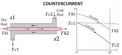
After making some assumptions, you can calculate the efficiency of heat transfer with this formula:
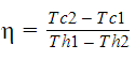
Where…
- ɳ is the efficiency of the heat transfer
- Tc2 is the the temperature of the cold stream at position x2.
- Tc1 is the temperature of the cold stream at position x1.
- Th1 is the the temperature of the hot stream at position x1.
- Th2 is the temperature of the hot stream at position x2.
You collect temperature reading from each sensor at 2 different times for a total of 8 points with the following schema:
- 1 bucket: sensors
- 4 measurements: Tc1, Tc2, Th1, Th2
- 1 Field: temperature
Since the temperature readings are stored in different measurements, you need to join the data in order to calculate the efficiency.
First, I want to gather the temperature readings for each sensor. I start with Th1. I need to prepare the data. I drop the “_start” and “_stop” columns because I’m not performing any group by’s or windowing. Dropping these columns is by no means necessary, it just simplifies the example. I will just be performing math across values on identical timestamps, so I keep the “_time” column.
Th1 = from(bucket: "sensors")
  |> range(start: -1d)
  |> filter(fn: (r) => r._measurement == "Th1" and r._field == "temperature")
  |> yield(name: "Th1")
| Not In Group Key | In Group Key | In Group Key | Not In Group Key | Not In Group Key |
| table | _measurement | _field | _value | _time |
| 0 | Th1 | temperature | 80.90 | rfc3339time1 |
| 0 | Th1 | temperature | 81.00 | rfc3339time2 |
Th2 = from(bucket: "sensors")
  |> range(start: -1d)
  |> filter(fn: (r) => r._measurement == "Th2" and r._field == "temperature")
  |> yield(name: "Th2")
| Not In Group Key | In Group Key | In Group Key | Not In Group Key | Not In Group Key |
| table | _measurement | _field | _value | _time |
| 0 | Th2 | temperature | 70.2 | rfc3339time1 |
| 0 | Th2 | temperature | 71.6 | rfc3339time2 |
Next, join the two tables.
TH = join(tables: {Th1: Th1, Th2: Th2}, on: ["_time","_field"])
| Not In Group Key | In Group Key | In Group Key | In Group Key | Not In Group Key | Not In Group Key | Not In Group Key |
| table | _measurement_Th1 | _measurement_Th2 | _field | _value_Th1 | _value_Th2 | _time |
| 0 | Th1 | Th2 | temperature | 80.90 | 70.2 | rfc3339time1 |
| 0 | Th1 | Th2 | temperature | 81.00 | 71.6 | rfc3339time2 |
The join() function takes a key table pair as input to the tables parameter and column names to the on parameter. The join() function only executes inner joins and joins all columns with equal values. The _time and _field columns have equal values where the _value and _measuremnt columns do not. The table key is appended to the column name to trace like columns with different values back to their input table. Any columns that aren’t included in the on parameter won’t be joined.
Next, apply this logic to the cold stream as well:
TC = join(tables: {Tc1: Tc1, Tc2: Tc2}, on: ["_time"])
| Not In Group Key | In Group Key | In Group Key | In Group Key | Not In Group Key | Not In Group Key | Not In Group Key |
| table | _measurement_Tc1 | _measurement_Tc2 | _field | _value_Tc1 | _value_Tc2 | _time |
| 0 | Tc1 | Tc2 | temperature | 50.50 | 60.3 | rfc3339time1 |
| 0 | Tc1 | Tc2 | temperature | 51.00 | 59.3 | rfc3339time2 |
Next, join TC with TH and calculate the efficiency. For the sake of simplicity we’ll drop the measurement columns as well.
THTC = join(tables: {TH: TH, TC: TC}, on: ["_time"])
|> drop( columns: ["_measurement_Th1","_measurement_Th2","_measurement_Tc1","_measurement_Tc2"])
|> yield(name: "TCTH")
| Not In Group Key | In Group Key | Not In Group Key | Not In Group Key | Not In Group Key | Not In Group Key | Not In Group Key |
| table | _field | _value_Th1 | _value_Th2 | _value_Tc1 | _value_Tc2 | _time |
| 0 | temperature | 80.90 | 70.2 | 50.50 | 60.3 | rfc3339time1 |
| 0 | temperature | 81.00 | 71.6 | 51.00 | 59.3 | rfc3339time2 |
Finally, I can use the map() to calculate the efficiency across all of the measurements. This is what the code looks like all together:
TCTH
|> map(fn: (r) => (r with efficiency: r._value_Tc2 - r._value_Tc1)/(r._value_Th1 - r._value_Th2)*100)
|> yield(name: "efficiency")
I can see that the heat transfer efficiency has decreased over time.
| Not In Group Key | In Group Key | Not In Group Key | Not In Group Key | Not In Group Key | Not In Group Key | Not In Group Key | Not In Group Key |
| table | _field | _value_Th1 | _value_Th2 | _value_Tc1 | _value_Tc2 | efficiency | _time |
| 0 | temperature | 80.90 | 70.2 | 50.50 | 60.3 | 92 | rfc3339time1 |
| 0 | temperature | 81.00 | 71.6 | 51.00 | 59.3 | 88 | rfc3339time2 |
Union
The union() function allows you to combine one more table stream which results in a table stream output with an increased table length. Union is frequently used to:
- Merge data across measurements or tags.
- Merge transformed data with the original data.
- Merge data with different time ranges to make data continuous.
For example imagine we had the following data:
| Not in Group Key | In Group Key | In Group Key | Not In Group Key | Not In Group Key |
| table | _measurement | _field | _value | _time |
| 0 | measurement1 | field1 | 1.0 | rcc3339time1 |
| 0 | measurement1 | field1 | 2.0 | rcc3339time2 |
| Not in Group Key | In Group Key | In Group Key | Not In Group Key | Not In Group Key |
| table | _measurement | _field | _value | _time |
| 0 | measurement2 | field2 | 4.0 | rcc3339time1 |
| 0 | measurement2 | field2 | 5.0 | rcc3339time2 |
| Not in Group Key | In Group Key | In Group Key | Not In Group Key | Not In Group Key |
| table | _measurement | _field | _value | _time |
| 0 | measurement3 | field3 | 3.0 | rcc3339time1 |
| 0 | measurement3 | field3 | 7.0 | rcc3339time2 |
For example we could uses array.from() to construct that example:
import "experimental"
import "array"

rfc3339time1 = experimental.subDuration(d: -1m, from: now())
rfc3339time2 = experimental.subDuration(d: -2m, from: now())

data1 = array.from(rows: [
{_time: rfc3339time1, _value: 1.0, _field: "field1", _measurement: "measurement1"},
{_time: rfc3339time2, _value: 2.0, _field: "field1", _measurement: "measurement1"}])

data2 = array.from(rows: [{_time: rfc3339time1, _value: 4.0, _field: "field2", _measurement: "measurement2"},
{_time: rfc3339time2, _value: 5.0, _field: "field2", _measurement: "measurement2"}])

data3 = array.from(rows: [{_time: rfc3339time1, _value: 4.0, _field: "field3", _measurement: "measurement3"},
{_time: rfc3339time2, _value: 5.0, _field: "field3", _measurement: "measurement3"}])
Now we might use union() to combine the three table streams together and pivot on the field and measurement:
union(tables: [data1, data2, data3])
|> yield(name:"after union")
|> pivot(rowKey:["_time"], columnKey: ["_field", "_measurement"], valueColumn: "_value")
|> yield(name:"after pivot")
Where the first yield() function returns “after union”:
| Not in Group Key | In Group Key | In Group Key | Not In Group Key | Not In Group Key |
| table | _measurement | _field | _value | _time |
| 0 | measurement1 | field1 | 1.0 | rcc3339time1 |
| 0 | measurement1 | field1 | 2.0 | rcc3339time2 |
| 0 | measurement2 | field2 | 4.0 | rcc3339time1 |
| 0 | measurement2 | field2 | 5.0 | rcc3339time2 |
| 0 | measurement3 | field3 | 3.0 | rcc3339time1 |
| 0 | measurement3 | field3 | 7.0 | rcc3339time2 |
The second yield() function returns “after pivot”
| Not in Group Key | In Group Key | In Group Key | Not In Group Key | Not In Group Key |
| table | _field1_measurement1 | _field2_measurement2 | _field3_measurement3 | _time |
| 0 | 1.0 | 4.0 | 3.0 | rcc3339time1 |
| 0 | 2.0 | 5.0 | 7.0 | rcc3339time2 |
Using union() and pivot in this way allows you to achieve a result similar to using a join() function. However, unlike the join() function, the union() function allows you to combine more than two tables together.
Accessing External Data Sources
You can use Flux to bring in data from a variety of other sources including SQL databases, other InfluxDB Cloud Accounts, Annotated CSV from a URL, and JSON.
The Flux SQL package
You can use the Flux SQL package to query and write to a variety of SQL data source including:
- Amazon RDS
- Athena
- Google BigQuery
- CockroachDB
- MariaDB
- MySQL
- Percona
- PostgreSQL
- SAP HANA
- Snowflake
- Microsoft SQL Server
- SQLite
Use the sql.from() function to query a SQL source. For example, to query a local Postgres instance use the following Flux query: import "sql"
sql.from(
  driverName: "postgres",
  dataSourceName: "postgresql://user:password@localhost",
  query:"SELECT * FROM TestTable"
)
Use the sql.to() function to write data to SQL database. For, example to write data to a local MySQL instance use the following Flux query:
import "sql"
data
|> sql.to(
  driverName: "mysql",
  dataSourceName: "username:password@tcp(localhost:3306)/dbname?param=value",
  table: "example_table",
  batchSize: 10000
)
Kee the following data requirements in mind when using the sql.to() function:
- Data in the steam must have the same column names as your SQL database. Use a combination of drop(), keep(), map(), and rename() to prepare your data before using the sql.to() function.
- Remember your SQL schema rules. All data that doesn’t conform to your SQL schema rules will be dropped. Use the map() function to conform data to our SQL schema rules.
CSV
You can use Flux to import a Raw CSV or Annotated CSV from a URL (or from a local file) with the csv.from() functions. There are two csv.from() functions:
- csv.from() from the Flux experimental CSV package which supports Annotated CSV
- csv.from() from stdlib which supports Annotated or Raw CSV
experimental csv.from()
Use the csv.from() function from the Flux experimental CSV package to retrieve an Annotated CSV from a URL. For example the NOAA water sample data pulls data from an Annotated CSV:
import "experimental/csv"

csv.from(url: "https://influx-testdata.s3.amazonaws.com/noaa.csv")
Note: You can also upload Annotated CSV from a local file with the csv.from() function stdlib with the Flux REPL. You need to build the Flux REPL from source and use it to access your local file system. This version of csv.from() also returns a stream of tables from Annotated CSV stored in a Flux variable.
csv.from()
Use the csv.from() function from stdlib to retrieve a Raw CSV from a URL. For example you can use the csv.from() function to parse CSV data from API and write it to InfluxDB in a task. A great example of this can be found in the Earthquake Feed Ingestion task from the Earthquake Command Center Community Template. Here is the relevant Flux from that task:
onedayago = strings.trimSuffix(v: string(v: date.truncate(t: experimental.subDuration(d: 1d, from: now()), unit: 1m)), suffix: ".000000000Z")
csv_data_url = "https://earthquake.usgs.gov/fdsnws/event/1/query?format=csv&starttime=" + onedayago + "&includedeleted=true&orderby=time-asc"
csv_data = string(v: http.get(url: csv_data_url).body)
states = ["Alaska", "California", "CA", "Hawaii", "Idaho", "Kansas", "New Mexico", "Nevada", "North Carolina", "Oklahoma", "Oregon", "Washington", "Utah"]
countries_dictionary = dict.fromList(pairs: [{key: "MX", value: "Mexico"}])

csv.from(csv: csv_data, mode: "raw")
First the user builds their URL. Since this is a task, or a Flux script that’s executed on a schedule, the user wants to build their URL with a dynamic starttime value. They use the experimental.Subduration() function to get the timestamp from -1d. Then they truncate the timestamp with date.truncate() to round the timestamp down to the last minute or ".000000000Z" . The string() function is used to convert the timestamp into a string and the strings.trimSuffix() function removes the subseconds to format the starttime into the required format as specified by the USGS Earthquake API. Next they use the http.get() function to submit an HTTP GET request to the USGS Earthquake API. Finally they use the csv.from() function to parse the CSV.
To learn about how to install a Community Template, please look at the
JSON
Use the json.parse() function from the Flux experimental JSON package to return values from a JSON. Like the example above, you can also use json.parse() with http.get() to parse a HTTP GET JSON response and convert it to a Flux table:
import "array"
import "experimental/json"
import "experimental/http"
resp = http.get(url: "https://api.openweathermap.org/data/2.5/weather?q=London,uk&APPID=0xx2")
jsonData = json.parse(data: resp.body)
array.from(rows: [{_time: now(), _value: float(v:jsonData.main.temp)}])
|> yield()
Which produces the following table:
| Not in Group Key | Not Iin Group Key | Not In Group Key |
| table | _value | _time |
| 0 | 285.33 | rcc3339time1 |
Where the OpenWeatherMap current weather data API yields the following HTTP GET JSON response:
{"coord":{"lon":-0.1257,"lat":51.5085},"weather":[{"id":801,"main":"Clouds","description":"few clouds","icon":"02n"}],"base":"stations","main":{"temp":285.33,"feels_like":284.67,"temp_min":282.94,"temp_max":287.35,"pressure":1024,"humidity":79},"visibility":10000,"wind":{"speed":2.11,"deg":254,"gust":4.63},"clouds":{"all":21},"dt":1633546918,"sys":{"type":2,"id":2019646,"country":"GB","sunrise":1633500560,"sunset":1633541256},"timezone":3600,"id":2643743,"name":"London","cod":200}
Materialized Views or Downsampling Tasks
Materialized views or downsampling is the process of converting high resolution data to lower resolution aggregates. Downsampling is an important practice in time series database management because it allows users to preserve disk space while retaining low precision trends of their data over long periods of time. Users typically apply an aggregate or selector function to their high resolution data to create a materialized view of a lower resolution summary:
- Flux built-in aggregate transformations like mean(), count(), sum() etc.
- Flux built-in selector transformations like max(), min(), median(), etc.
To downsample the data temperature from the Air Sensor sample dataset, you might perform the following query: \
from(bucket: "airsensor")
  |> range(start: -10d)
  |> filter(fn: (r) => r["_measurement"] == "airSensors")
  |> aggregateWindow(every:1d, fn: mean, createEmpty: false)
  |> to(bucket: "airSensors_materializedView"0
Use the to() function to write the data to a destination bucket. Destination buckets usually have a longer retention policy than the source bucket to conserve on disk space. Running this query will write the materialized view to the “airSensors_materializedView” bucket once. However, users typically perform downsampling on a schedule, or a task. Using tasks to create materialized views will be covered in detail in Part 3.
Further Reading
- TL;DR InfluxDB Tech Tips: Multiple Aggregations with yield() in Flux
- TL;DR InfluxDB Tech Tips – Aggregating across Tags or Fields and Ungrouping
- TL;DR InfluxDB Tech Tips: Parameterized Flux Queries with InfluxDB
- https://www.influxdata.com/blog/top-5-hurdles-for-intermediate-flux-users-and-resources-for-optimizing-flux/
- Top 5 Hurdles for Flux Beginners and Resources for Learning to Use Flux
- TL;DR InfluxDB Tech Tips – From Subqueries to Flux!
- TL;DR InfluxDB Tech Tips – How to Extract Values, Visualize Scalars, and Perform Custom Aggregations with Flux and InfluxDB
- TL;DR Tech Tips – How to Construct a Table with Flux
- Anomaly Detection with Median Absolute Deviation