Designing Your Schema
Table of contents
- General Recommendations for Schema Design and Data Layout
- Series Cardinality
- Runaway Cardinality
- Using Tags Intelligently
- Data Partitioning
- Metrics vs. Events
- Enforcing a Schema
Figuring out the best data layout or schema for InfluxDB is important in optimizing the resources used by InfluxDB, as well as improving ingestion rates and the performance of Flux queries and tasks (scheduled Flux scripts). You also want to consider developer experience when designing your schema.
General Recommendations for Schema Design and Data Layout
Generally, you should abide by the following recommendations when designing your schema:
- Keep bucket and measurement names short and simple.
- Avoid encoding data in measurement names.
- Encode meta data in tags.
- Commonly queried metadata should be stored in tags for better query performance because tags are indexed while field values are not indexed.
- Limit the number of series or try to reduce series cardinality and avoid runaway series cardinality.
- Separate data into different buckets when you need to either:
- assign different retention policies to that data.
- or need to scope authentication token to that bucket.
Series Cardinality
Series cardinality is the number series in your InfluxDB instance. Remember, a series is defined by the unique combinations of measurements, tag sets, and fields. Part of the reason why InfluxData adopted the “schema on write” approach for InfluxDB is because series creation and the resulting indexing generally offers efficient queries. However, this is only true up to a point. Similar to an over-indexed relational database, it can be possible for too much cardinality to slow down writes and queries because the indexes tracking the groups get too large.
How much cardinality is too much? There is no single answer for that. However, each free tier user is currently limited to 10,000 total cardinality in their whole InfluxDB Cloud account. Pay as You Go (PaYG) customers are limited to 1,000,000 cardinality total.
How to estimate Cardinality
To estimating your cardinality:
- Multiply the possible tag values for each possible tag for a worst case estimate.
- Multiply the value in step 1 by the number of fields for a worse case estimate.
- Repeat steps 1 and 2 for each measurement and each bucket, and then sum all of the values.
In other words, the worst-case cardinality for a measurement = number of tag keys * number of tag values * number of field keys. The reason that this is “worst-case” is because it overestimates the total series in the presence of dependent tags. The worst-case cardinality equation assumes that every tag set is unique. In reality sometimes tags are redundant or dependent.
Dependent Tags
A dependent tag is scoped by another tag. Dependent tags don’t influence the series cardinality, and should be removed from the cardinality calculation. Let’s take a look at the following line protocol to demonstrate how a dependent tag doesn’t influence the series cardinality.
measurement1,tag1="tagvalue1",tag2="tagvalue3" field1=1i,field2=1,field3="a" unixtime1
measurement1,tag1="tagvalue2",tag2="tagvalue4"  field1=2i,field2=2,field3="b" unixtime2
measurement1,tag1="tagvalue1",tag2="tagvalue3" field1=1i,field2=1,field3="a" unixtime3
measurement1,tag1="tagvalue2",tag2="tagvalue4"  field1=2i,field2=2,field3="b" unixtime4
In this instance the “tag2” tag key is a dependent tag because its tag value is dependent on the value of the “tag1” tag key. In other words, every time the value of the “tag1” tag key is “tagvalue1” the value of the “tag2” tag key is “tagvalue3”. Similarly, every time the “tag1” tag key is “tagvalue2” the value of the “tag2” tag key is “tagvalue4”. In this way “tag2” is scoped by “tag1”. If we were to calculate the series cardinality without removing the dependent tag, “tag2” we would get:
1 measurement x ( 2 tag values for “tag1” x 2 tag values for “tag2”) x** 3** fields = 12 overestimated series cardinality
Again, each series is identified by their unique tag keys, tag values, and field key combinations. Because a series is defined in part by a unique set of tag values, in this case, the introduction of tag2 does not change the table or series count in the underlying data model. Therefore to correctly calculate the series cardinality, **remove **the dependent tag, “tag2” from the equation:
1 measurement x 2 tag values for “tag1” x** 3** fields = 6 actual series cardinality
Runaway Cardinality
While calculating series cardinality can be challenging, accidentally overestimating your series cardinality shouldn’t be a real concern of yours – after all, InfluxDB has tools which calculate your cardinality for you (more on that later). However, you do need to make sure to avoid runaway cardinality. Runaway series cardinality occurs when you load your tags or measurements with data that is potentially unbounded. To illustrate a runaway series cardinality scenario, consider the following hypothetical situation in which we’re building an IoT application on top of InfluxDB. For this hypothetical IoT application example we’re gathering the following data:
- We have a set of customers. Each customer is identified with a single “customer_id” tag value under the “customer_id” tag key.
- Each customer has a number of devices. Each one of the customer’s devices is identified with device id tag values under the “device_id” tag key.
- Each device reports fields.
For this example, cardinality = Cn _ * _Dn * F
Where…
_Cn = the number of “customer_id” tag values _
Dn = the number of “device_id” tag values
_F = the number of field keys _
Assuming your customers continue to grow, you can see how cardinality may “explode”. For example, if you start with 5 customers each with 5 devices, each with 1 field, total cardinality is 5 * 5 * 1, or a mere 25. However, if you end up with 100,000 customers, with 10 devices each, each with 5 fields, you end up with 100,000 * 10 * 5, or 5,000,000. Whoops, you blew your cardinality limit!
Causes
The most common schema design mistakes that can lead to runaway cardinality are:
Mistake 1: Log messages as tags.
Solution 1: We don’t advise that anyone store logs as tags due to the potential for unbounded cardinality (e.g. logs likely contain unique timestamps, UUIDs, etc). You can store attributes of a log as a tag, as long as the cardinality isn’t unbounded. For example, you could extract the log level (error, info, debug) or some key fields from the log message. Storing logs as a field is ok, but it is less efficient to search (essentially table scans), compared to other solutions.
Mistake 2: Too many measurements. This typically happens when people are moving from —or think of InfluxDB as— a key-value store. So for example, if you’re writing system stats to an InfluxDB instance you might be inclined to write data like so: Cpu.server-5.us-west.usage_user value=20.0
Solution 2: Instead encode that information as tags like so: cpu, host=server-5, region = us-west, usage_user=20.0
Mistake 3: Making ids (such as eventid, orderid, etc…) a tag. This is another example that can cause unbounded cardinality if the tag values aren’t scoped.
Solution 3: Instead, make these metrics a field.
Using Tags Intelligently
Understanding how to properly use tags can not only help prevent runaway series cardinality but also increase your Flux query performance. In this section, we’ll refer to the Air sensor sample dataset to illustrate how to use tags intelligently. The Air sensor sample dataset represents an IoT use case. It contains the following schema:
- 1 measurement: airSensors
- 3 fields: co, humidity, temperature,
- 1 tag key: sensor_id
- 8 tag values: TLM0100, TLM0101, TLM0102, TLM0103, TLM0200, TLM0101, TLM0202, TLM0203
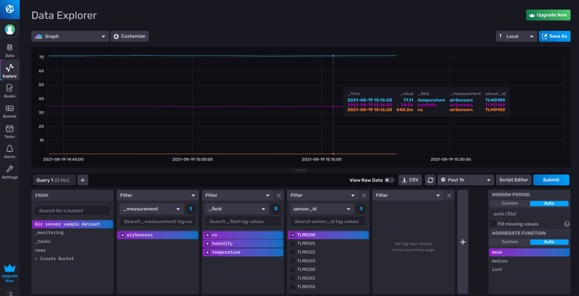 Visualizing co, humidity, and temperature for th TLM0100 sensor from the Air sensor sample dataset after writing it to InfluxDB with the to() function as described in Write and Query Sample Data.
Just Enough Flux
So far we have only discussed querying InfluxDB in an abstract manner. In order to understand the impact that tags have on Flux query performance, we need to take a moment to learn some Flux basics. This section is a crash course on Flux, the query, data transformation, and scripting language for InfluxDB 2.0. The aim of this section is to provide you with just enough basic understanding of Flux to be able to interpret the examples. We’ll deep dive into the Flux language in the following chapter.
from() |> range() |> filter()
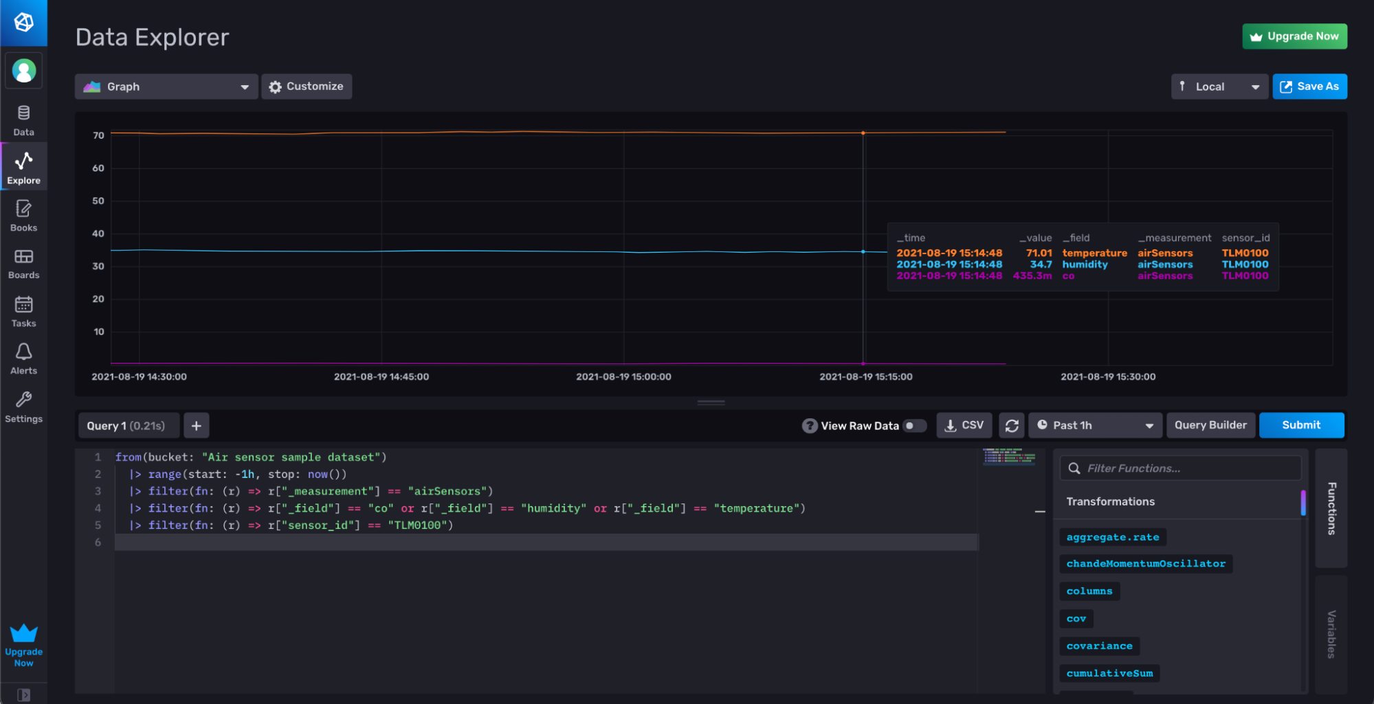
The following Flux query queries for the co, humidity, and temperature fields from the TLM0100 sensor from the Air sensor sample dataset bucket.
from(bucket: "Air sensor sample dataset")
|> range(start: -1h, stop: now())
|> filter(fn: (r) => r["_measurement"] == "airSensors")
|> filter(fn: (r) => r["_field"] == "co" or r["_field"] == "humidity" or r["_field"] == "temperature")
|> filter(fn: (r) => r["sensor_id"] == "TLM0100")
The most basic Flux queries contain three functions:
- The from() function. A Flux query typically starts with a from() function. This function retrieves data from a specified bucket.
- The range() function. The range() function must follow the use of a from() function. The range() function filters records based on time bounds provided to the start and stop parameters.
- You can pass relative durations (see the example above), absolute time (2019-08-28T22:00:00Z) , or integers (1567029600) into the start and stop parameters.
- The filter() function. The filter() function filters records based on conditions specified in the predicate function,
fn. You can use the filter function() to filter for specific measurements, tags, and fields. You can also use the filter function to filter values based on thresholds and apply conditional query logic. The order of subsequent filter() functions doesn’t have an impact on performance.
In Flux, functions are connected together through the |> pipe-forward operator.
The Purpose of Tags
As covered in the previous section, tag keys are grouped by the storage engine based on series. This allows the storage engine to quickly find points based on the tag keys and fields rather than scanning through all of your data to find the results of a query.
To illustrate how indexing improves query performance, let’s consider the Air sensor sample dataset. Remember, the specific sensors that gather air quality data are tagged with a “sensor_id”. Now imagine that you want to query the dataset for all of the data from a specific sensor with a unique “sensor_id” value. When you apply a filter to query for a single tag value, the storage engine can use the indexed tag to quickly find the relevant table in the storage engine and return all the data associated with that tag value quickly.
 Filtering for a TLM0100 tag value from the “sensor_id” tag.
Incorrectly casting tags as fields for the Air Quality dataset
However, if “sensor_id” was a field instead of a tag, then that sensor id isn’t indexed. Therefore, the storage engine would pull from one massive table for all of the sensor ids, using only the timestamps in the range() function as direction for which subset of data to pull from. In that instance, the storage engine would have to scan through all of the rows of that one massive table in order to pull out the rows that match the specific sensor id field value we’re filtering for. This scanning and row selection process is far less efficient than simply streaming out the relevant tables in their entirety.
Casting the sensor id as a field presents additional query challenges and performance problems. Most likely you obtain senor id data because you want to know what the humidity or temperature is for a specific sensor. However, querying for the temperature from a specific sensor becomes extra challenging if your sensor id is a field. You would have to:
- Query for the sensor id field values.
- Query for the temperature field values.
- Join those two query results on timestamp–**assuming **that you only have one sensor reporting temperature values at each timestamp.
In other words if the “sensor_id” was a field instead of a tag and you wanted to query for the temperature from that sensor you would have to query for the following 2 tables first:
| _measurement | _field | _value | _time |
| airSensors | sensor_id | TLM0100 | rfc3339time1 |
| airSensors | sensor_id | TLM0100 | rfc3339time2 |
| airSensors | sensor_id | TLM0101 | rfc3339time3 |
| airSensors | sensor_id | TLM0101 | rfc3339time4 |
| _measurement | _field | _value | _time |
| airSensors | temperature | 73.57230556533555 | rfc3339time1 |
| airSensors | temperature | 71.2194835668512 | rfc3339time2 |
| airSensors | temperature | 71.80350992863588 | rfc3339time3 |
| airSensors | temperature | 71.78232293801005 | rfc3339time4 |
To find the temperatures for the sensor TLM0100 the storage engine would need to read through the first table and pull out rows that have a _value of “TLM0100” then find matching timestamps in the second table and then merge those two tables and return them. When those tables become millions of rows long, you can see how this can slow down response time.
Correctly using tags for the Air Quality Dataset
All of the problems in the section above are avoided when the sensor id is a tag. When you filter for the temperature for a specific “sensor_id” tag value, the storage engine simply reads out the first table as listed below because that series is indexed. The storage engine is able to return all the temperature results for a specific “sensor_id” even if the table has millions of rows (or the series has millions of points).
| _measurement | sensor_id | _field | _value | _time |
| airSensors | TLM0100 | temperature | 73.57230556533555 | rfc3339time1 |
| airSensors | TLM0100 | temperature | 71.2194835668512 | rfc3339time2 |
| _measurement | sensor_id | _field | _value | _time |
| airSensors | TLM0101 | temperature | 71.80350992863588 | rfc3339time1 |
| airSensors | TLM0101 | temperature | 71.78232293801005 | rfc3339time2 |
The Purpose of Measurements
As covered in the previous section, measurements are grouped by the storage engine based on series. This allows the storage engine to quickly find points based on the measurements rather than scanning through all of your data to find the results of a query. The purpose of measurements is similar to the purpose of tags, but measurements offer a higher level of organization to your data. If your fields or tags are related, they should go into one measurement. Writing related data to the same measurement helps you avoid having to query for multiple measurements and perform joins. For example, imagine we’re developing a human health app and gathering blood oxygen levels, heart rate, and body temperature data. I would write the blood oxygen level, heart rate, and body temperature fields to one measurement because I foresee needing to simultaneously visualize and compare a combination of the metrics to assess human health. While you could separate out the fields into different measurements for a human health app, you’d most likely have to use joins() to perform math across measurements which are more computationally expensive.
Data Partitioning
The final consideration for schema design in InfluxDB is finding the best approach to bucket and org data partitioning, especially when developing a customer facing IoT application on top of InfluxDB. There are 3 options:
- Single Bucket
- Bucket per User
- Org per Customer
Remember authentication tokens can be restricted to read or write from individual buckets. Additionally each bucket is assigned one retention policy. Like tags and measurements, buckets are also indexed.
Single Bucket
The single bucket design has the following advantages:
- Writing all of your data to a single bucket makes querying for data easier. You don’t have to keep track of which data exists within multiple buckets. You’ll likely need to use multiple measurements to organize your data effectively. However, you can still easily perform aggregations across multiple measurements by grouping the measurements together.
- You can perform one downsampling task to downsample all of your data. Downsampling tasks are used to reduce the overall disk usage of your data by transforming high resolution data into lower resolution aggregates.
The single bucket design has the following disadvantages:
- Each bucket is assigned one retention policy. With this design you can’t expire data subsets at different retention intervals.
- If you need to query for a invicidual user’s data within a single bucket for your application, you should generate new read tokens for each individual customer. However, this design is less secure against malicious attacks than isolating different users’ data in separate buckets.
The single bucket approach is good for use cases where:
- You’re developing a simple IoT application, like the Air sensor sample dataset.
- You intend on treating all of your user’s data in the same way. Your data is being collected at similar intervals and a single retention policy is an effective solution for proper time series database management.
- Your data is relatively non-sensitive and preventing a data breach is of little or no concern.
Bucket per User
The bucket per user design has the following advantages:
- Your customer’s data is isolated and secure.
- You can assign different retention policies to your different buckets depending on your customer’s needs.
The bucket per user design has the following disadvantages:
- You can’t visualize multiple users’ data without joining the data across the buckets first.
- Performing math across your users’ data is hard. For example if you want to know which user is reporting a max value for their field, you must first join all of your data together across the different user buckets first.
- You’ll likely need to write multiple downsampling tasks to downsample all of your user’s data. You can automate some of this downsampling task creation with the use of parameterized queries, but it’ll require a little more work.
The bucket per user design is good for use cases where:
- You’re developing a more sophisticated IoT application and the data is sensitive, like a human health application.
- You’re writing sensitive data to InfluxDB and isolating your users’ data is a priority.
- Your customers have different data requirements and you need to provide them with different time series data management solutions (including different retention policies and downsampling tasks).
Org per Customer
The org per customer design has the following advantages:
- You can meet the data requirements of users with advanced high throughput and cardinality use cases.
- Your users’ data is isolated and secure.
The org per customer design has the following disadvantage:
- You can’t easily query for data across multiple organizations.
The org per customer design is good for use cases where:
- You’re developing an industrial IoT solution that can be used for multiple companies.
Metrics vs. Events
Understanding the difference between metrics and events is helpful for designing your schema. Metrics are time series data collected at regular intervals. Metrics are typically pulled from the data source. Metrics usually require regular downsampling tasks to convert the high resolution data to lower resolution aggregates for efficient disk usage management.
Events are metrics collected at irregular intervals. They are typically pushed from the data source. A common design for industrial IoT application development is to write metrics from an IoT device to an OSS InfluxDB instance at the edge or in the fog. Then when those metrics meet certain conditions those events get pushed to the cloud.
Metrics have an advantage over events, in that if metrics are written at precisely the same time intervals, the InfluxDB storage engine can apply aggressive compression when writing those metrics to disk. For Cloud, this will result in a small advantage in terms of read performance. For OSS users, this will also mean that you will be using less disk for the same metrics.
Enforcing a Schema
Enforcing a schema with InfluxDB is important for maintaining consistent writes and for preventing data injections or bad writes. You can enforce a schema at the bucket level with explicit bucket schemas. You have to use the CLI to create a bucket with an explicit schema. First create a bucket with the influxd bucket create command and specify an explicit schema.
influx bucket create \
  --name "Air sensor sample dataset"\
  --schema-type explicit
Next create a schema columns file for each measurement you want to add. We’ll enforce a schema for our airSensors measurement for our Air sensor sample dataset. Our schema columns file will be a CSV, but you can use JSON or NDJSON. Name the schema columns file (“airSensors_schema.csv”) and save it to your desired path.
name,type,data_type
time,timestamp,
sensor_id,tag,
co,field,float
humidity,field,float
temperature,field,float
Now we can add the schema to our airSensor measurement with the influx bucket-schema create command:
influx bucket-schema create \
 --bucket "Air sensor sample dataset" \
 --name airSensors \
 --columns-file airSensors_schema.csv
Specify the bucket that you want to create the schema for, the measurement to which your schema columns file should be applied to, and the path to your schema columns file.
Further Reading
- Data Layout and Schema Design Best Practices for InfluxDB
- InfluxDB schema design and data layout
- Solving Runaway Series Cardinality When Using InfluxDB
- Resolve high series cardinality 5.