Optimizing Flux Performance
Table of contents
- Optimizing Flux Performance
- General recommendations for Flux performance optimization
- Taking advantage of pushdown patterns
- Using schema mutations properly
- Using variables to avoid querying data multiple times
- Dividing processing work across multiple tasks
- The Flux Profiler package
- Using the Flux extension for Visual Studio Code to streamline Flux optimization discovery
- Other tips
- Best practices for receiving help
- Further Reading
Optimizing Flux Performance
So you’re using InfluxDB Cloud and you’re taking full advantage of Flux to create custom data processing tasks, checks, and notifications. However, you notice that some of your Flux scripts aren’t executing as quickly as you expect. In this section, we’ll learn about best practices and tools for optimizing Flux performance.
General recommendations for Flux performance optimization
Before diving into some of the tools you can use to optimize Flux performance, let’s dive into some general recommendations for Flux performance optimization:
- Take advantage of pushdown patterns.
- Schema mutation functions should be applied at the end of your query.
- Use variables to avoid querying data multiple times.
- Divide processing work across multiple tasks when needed.
We’ll discuss each of these recommendations in detail in the following sections.
Taking advantage of pushdown patterns
In order to provide context for the optimization guidelines, let’s first take a moment to understand how Flux works. Flux is able to query data efficiently because some functions push down the data transformation workload to storage rather than performing the transformations in memory. Combinations of functions that do this work are called pushdown patterns. It’s best to try and use pushdown patterns whenever you can in order to optimize your Flux query. To learn more about pushdown patterns and how Flux works, please read “Solution 2: Learning about memory optimizations and new pushdown patterns to optimize your Flux scripts” from Top 5 Hurdles for Intermediate Flux Users and Resources for Optimizing Flux.
Using schema mutations properly
Schema mutation functions are any functions that change the columns in your Flux tables. They include functions like keep(), drop(), rename(), duplicate(), and set(). If you’re using an aggregates or selector function in your query, try to include the schema mutation functions after applying aggregation functions to preserve any pushdown patterns that you might have. Additionally, try replacing keep() or drop() with changes to the group key whenever possible. For example, when executing a join() across two fields from two buckets, join on all the like-columns instead of dropping the columns afterwards. We generate the data for this example with the array.from() function:
import "array"
import "experimental"
start = experimental.subDuration(
d: -10m,
from: now(),
)
bucket1 = array.from(rows: [{_start: start, _stop: now(), _time: now(),_measurement: "mymeas", _field: "myfield", _value: "foo1"}])
|> yield(name: "bucket1")


bucket2 = array.from(rows: [{_start: start, _stop: now(), _time: now(),_measurement: "mymeas", _field: "myfield", _value: "foo2"}])
|> yield(name: "bucket2")
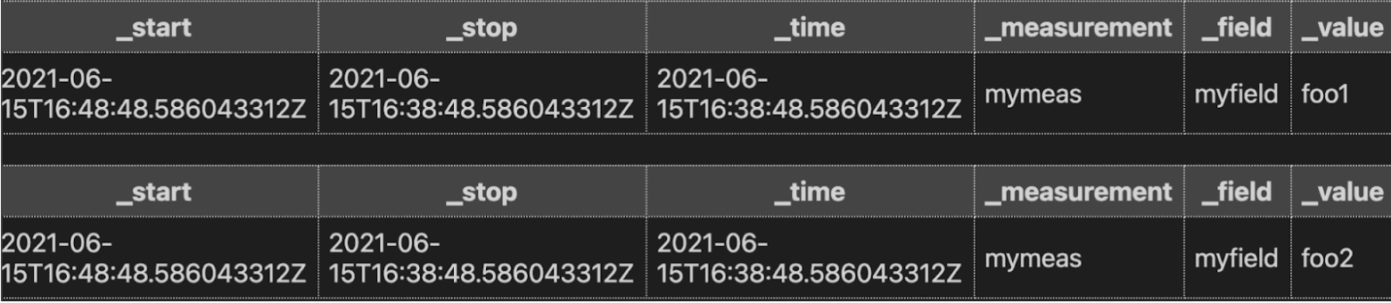
The annotated CSV output from our query looks like this:
Don’t use drop() unnecessarily after a join():
join(tables: {bucket1: bucket1, bucket2: bucket2}, on: ["_time"], method: "inner")
|> drop(columns:["_start_field1", "_stop_field1", "_measurement_field1", "myfield1"])
|> yield(name: "bad_join")
Do replace with changes to the group key by joining on like-columns:
join(tables: {bucket1: bucket1, bucket2: bucket2}, on: ["_start","_stop""_time", "_measurement","_field"], method: "inner")
|> yield(name: "good_join")
To yield the same result:

Using variables to avoid querying data multiple times
Rather than query data multiple times, store the result in a variable and reference it. In other words:
Don’t do this:
from(bucket: "my-bucket")
|> range(start: -1h)
|> filter(fn: (r) => r._measurement == "my_measurement")
|> mean()
|> set(key: "agg_type",value: "mean_temp")
|> to(bucket: "downsampled", org: "my-org", tagColumns:["agg_type"])

from(bucket: "my-bucket")
|> range(start: -1h)
|> filter(fn: (r) => r._measurement == "my_measurement")
|> count()
|> set(key: "agg_type",value: "count_temp")
|> to(bucket: "downsampled", org: "my-org", tagColumns: ["agg_type"])
Do this instead:
data = from(bucket: "my-bucket")
|> range(start: -1h)
|> filter(fn: (r) => r._measurement == "my_measurement")

data
|> mean()
|> set(key: "agg_type",value: "mean_temp")
|> to(bucket: "downsampled", org: "my-org", tagColumns: ["agg_type"])

data
|> count()
|> set(key: "agg_type",value: "count_temp")
|> to(bucket: "downsampled", org: "my-org", tagColumns: ["agg_type"])
Dividing processing work across multiple tasks
Are you trying to perform schema mutations, pivots, joins, complex math, and mappings all in the same task? If you are and you’re experiencing a long execution time, consider splitting up some of this work across multiple tasks instead. Separating the processing work out and executing these tasks in parallel can help you reduce your overall execution time.
The Flux Profiler package
The Flux Profiler package provides performance information based on your query. As per the documentation, the following Flux query:
import "profiler"

option profiler.enabledProfilers = ["query", "operator"]

from(bucket: "noaa")
  |> range(start: 2019-08-17T00:00:00Z, stop: 2019-08-17T00:30:00Z)
  |> filter(fn: (r) =>
    r._measurement == "h2o_feet" and
    r._field == "water_level" and
    r.location == "coyote_creek"
  )
  |> map(fn: (r) => ({ r with
    _value: r._value * 12.0,
    _measurement: "h2o_inches"
  }))
  |> drop(columns: ["_start", "_stop"])
Yields the following tables from the Profiler:
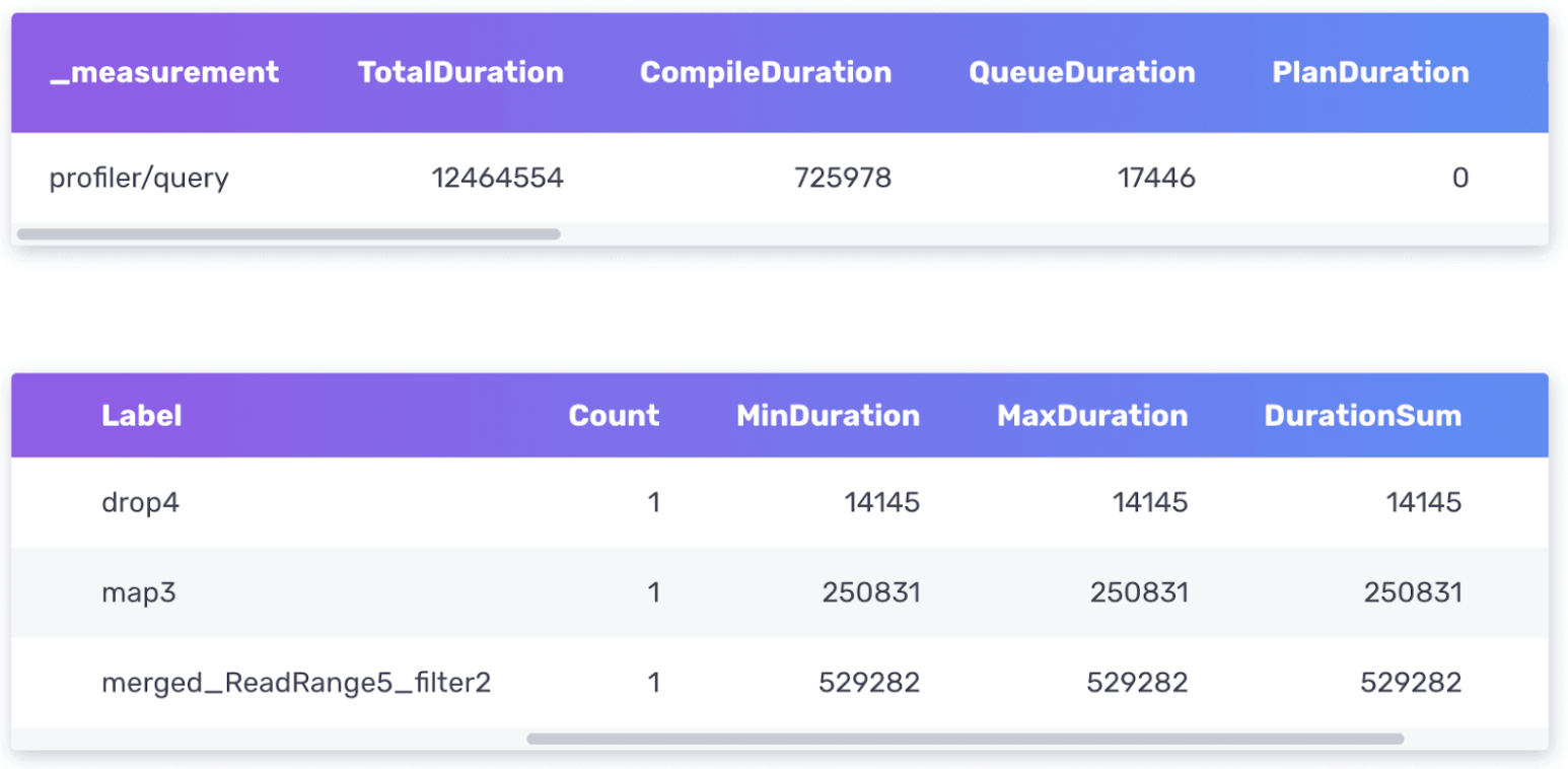
The Flux Profiler outputs performance information about your query in nanoseconds.
- The first table provides information about your entire query including the total duration time it took to execute the query as well as the time it spent compiling, in the queue, etc.
- The second table provides information about where the query is spending the most amount of time.
The two most important columns to pay attention to are the TotalDuration column from the first table and the DurationSum column from the second table. This query is executed very quickly, so I don’t have to worry about optimizing it. However, I’ll describe the thought process for optimizing it further.
First I would try to identify which part of the query is taking the longest to execute. From the query above, we can see that the merged_ReadRange5_filter operation has the largest DurationSum of 529282 ns. If I was planning to convert this query to a task and perform this transformation work on a schedule, the first thing I should consider is querying data over a shorter range and running the task more frequently.
Next, I notice that the map() function contributes the second longest DurationSum value. Taking a look back at my map() function, I have to wonder if renaming the measurement with map() is the most efficient way. Perhaps I should try using the set() function instead like so:
from(bucket: "noaa")
  |> range(start: 2019-08-17T00:00:00Z, stop: 2019-08-17T00:30:00Z)
  |> filter(fn: (r) =>
    r._measurement == "h2o_feet" and
    r._field == "water_level" and
    r.location == "coyote_creek"
  )
 |> drop(columns: ["_start", "_stop"])
  |> set(key: "_measurement",value: "h2o_inches")
  |> map(fn: (r) => ({ r with
    _value: r._value * 12.0,
  }))
Also notice that I switch the order of the functions and apply drop() and set() functions before the map() function. After running the Profiler, I see a decrease in the TotalDuration time which indicates that these were all good changes. Since performance optimizations are continuously made to Flux and everyone’s schema is very different, there aren’t hard rules for Flux performance optimization. Instead, I encourage you to take advantage of the Profiler and perform some experimentation to find solutions that work best for you.
Using the Flux extension for Visual Studio Code to streamline Flux optimization discovery
If you haven’t given it a try already, I encourage you to install the Flux extension for Visual Studio Code. To query your InfluxDB Cloud account with the Flux extension, you must first configure it and connect to your cloud account. I enjoy using the Flux extension and VS Code when trying to debug complicated Flux scripts or trying to optimize the performance of my Flux scripts because I can save my Flux scripts and compare outputs from the Profiler simultaneously.
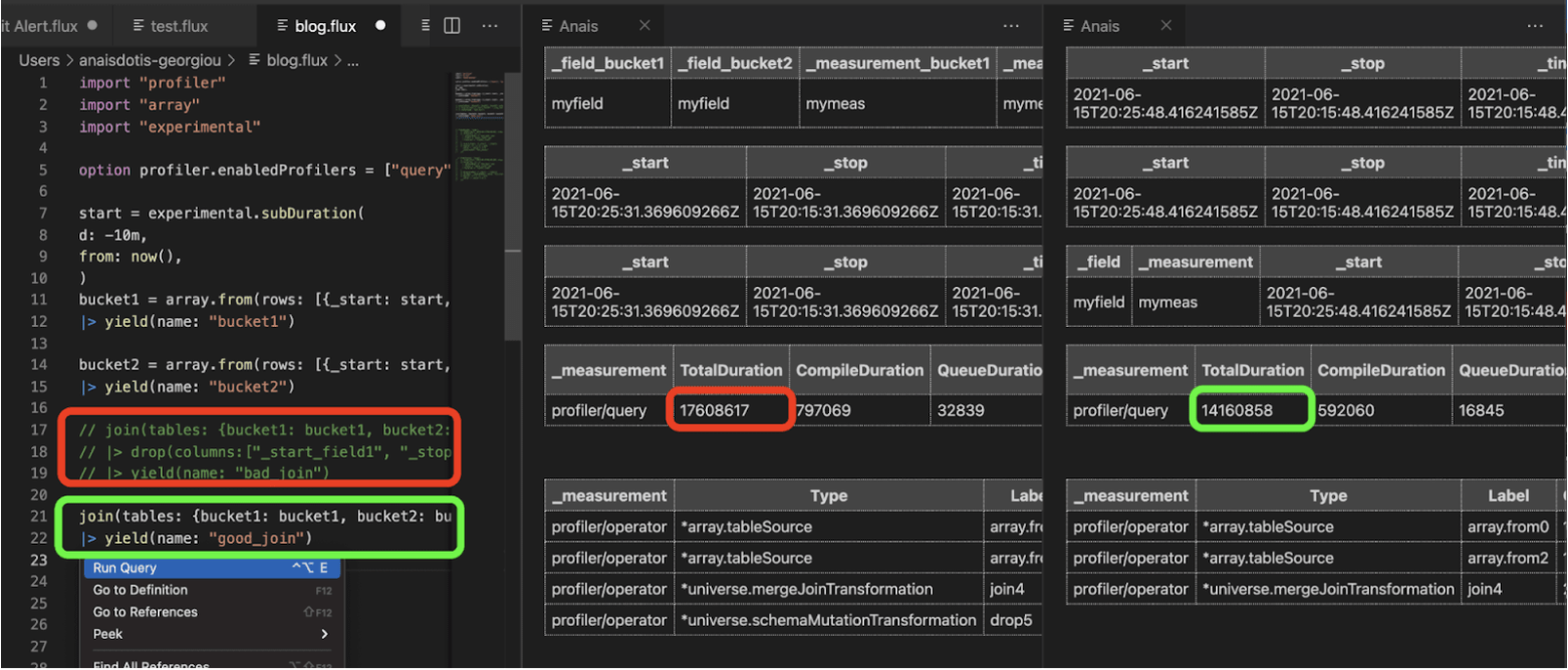
The original “bad_join” query (red) is commented out because I ran it first. Its TotalDuration time was 17608617 ns. Joining on multiple like-columns and removing the drop() improves the performance to 14160858 ns.
I decided to test the queries described in the “Using schema mutations properly” section above. The Profiler confirms my hypothesis: joining on multiple like-columns is more efficient than dropping redundant ones retroactively. While you can also perform this work in the InfluxDB UI, I find the side-by-side comparison of Profiler outputs helpful for this type of experimentation.
Other tips
Here are a list of other substitutions or ideas to consider when trying to optimize the performance of your Flux query:
- Can you use the experimental.join() function instead of join() function?
- Can you apply any groups that will reduce the number of rows in your table(s) before applying a map() function?
- Can you tune any regexes to be as specific as possible?
- Can you use rows.map() instead of map()?
- Does
|> sort(columns: ["_time"], desc: false) |> limit(n:1)perform better than|> last()?
Best practices for receiving help
When asking for help with optimizing the performance of your Flux script, whether it’s on the community forums, Slack, or through support, please include the following information in your post or request:
- What is the query that’s having an issue?
- Make sure to share it as well as including the output from the Profiler.
- What is the cardinality of your data? (how many series)
- Try using the InfluxDB Operational Monitoring Template to help you find the cardinality of your data.
- Alternatively try using the schema.cardinality() function to help you find the cardinality of your data.
- What is the density of your data? (how many points per unit time in each series)
- Try using the InfluxDB Cloud Usage Template to help you identify the data into your InfluxDB Cloud account.
- General information about how your data is structured (which measurements, fields and tag keys exist) is always helpful.
- Try using the schema package to share your data structure.
- What is your expectation of how fast a query should run? What’s the basis for that expectation?
Including as much of this information in a post will help us assist you better and more quickly. The above points also apply to issues with hitting memory limits.